10.1 Forward Euler method
Integrating the ODE
y ( t ) = y ( t 0 ) + ∫ t 0 t f ( τ , y ( τ ) ) d τ y(t) = y(t_0) + \int_{t_0}^t f(\tau, y(\tau)) \ud \tau y ( t ) = y ( t 0 ) + ∫ t 0 t f ( τ , y ( τ )) d τ We cannot find y ( t ) y(t) y ( t ) t t t t t t h h h
t 0 , t 0 + h , t 0 + 2 h , … t 0 , t 1 , t 2 , … \begin{align*}
& t_0, t_0+h, t_0+2h, \ldots \\
& t_0, t_1, t_2, \ldots
\end{align*} t 0 , t 0 + h , t 0 + 2 h , … t 0 , t 1 , t 2 , … i.e.,
t n = t 0 + n h , n = 0 , 1 , 2 , … t_n = t_0 + n h, \qquad n=0,1,2,\ldots t n = t 0 + nh , n = 0 , 1 , 2 , … Then
y ( t 1 ) = y ( t 0 ) + ∫ t 0 t 1 f ( τ , y ( τ ) ) d τ ≈ y ( t 0 ) + ∫ t 0 t 1 f ( τ , y ( t 0 ) ) d τ = y 0 + h f ( t 0 , y 0 ) \begin{align*}
y(t_1) &= y(t_0) + \int_{t_0}^{t_1} f(\tau, y(\tau)) \ud \tau \\
&\approx y(t_0) + \int_{t_0}^{t_1} f(\tau, y(t_0)) \ud \tau \\
&= y_0 + h f (t_0, y_0)
\end{align*} y ( t 1 ) = y ( t 0 ) + ∫ t 0 t 1 f ( τ , y ( τ )) d τ ≈ y ( t 0 ) + ∫ t 0 t 1 f ( τ , y ( t 0 )) d τ = y 0 + h f ( t 0 , y 0 ) We obtain the approximation
y 1 = y 0 + h f ( t 0 , y 0 ) y_1 = y_0 + h f(t_0, y_0) y 1 = y 0 + h f ( t 0 , y 0 ) This procedure can be continued to produce approximations at t 2 , t 2 , … t_2, t_2, \ldots t 2 , t 2 , …
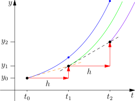
y n + 1 = y n + h f ( t n , y n ) , n = 0 , 1 , 2 , … y_{n+1} = y_n + h f(t_n, y_n), \qquad n=0,1,2,\ldots y n + 1 = y n + h f ( t n , y n ) , n = 0 , 1 , 2 , … 10.1.1 Geometric interpretation ¶ Through the point ( t 0 , y ( t 0 ) ) (t_0, y(t_0)) ( t 0 , y ( t 0 )) ( t 1 , y 1 ) (t_1, y_1) ( t 1 , y 1 ) y 1 = y 0 + h f 0 y_1 = y_0 + h f_0 y 1 = y 0 + h f 0
Now through the point ( t 1 , y 1 ) (t_1, y_1) ( t 1 , y 1 ) ( t 2 , y 2 ) (t_2, y_2) ( t 2 , y 2 )
This process is continued until we reach the final time.
10.1.2 Implementation ¶ The following function implements Euler method.
y n = y n − 1 + h f ( t n − 1 , y n − 1 ) y_n = y_{n-1} + h f(t_{n-1},y_{n-1}) y n = y n − 1 + h f ( t n − 1 , y n − 1 ) def euler(f,t0,T,y0,h):
N = int((T-t0)/h)
y = zeros(N)
t = zeros(N)
y[0] = y0
t[0] = t0
for n in range(1,N):
y[n] = y[n-1] + h*f(t[n-1],y[n-1])
t[n] = t[n-1] + h
return t, y
Consider the ODE problem
y ′ = y , t ≥ 0 y ( 0 ) = 1 \begin{align}
y' &= y, \qquad t \ge 0 \\
y(0) &= 1
\end{align} y ′ y ( 0 ) = y , t ≥ 0 = 1 whose exact solution is
y ( t ) = exp ( t ) y(t) = \exp(t) y ( t ) = exp ( t ) Right hand side function and exact solution
def f(t,y):
    return y

def yexact(t):
    return exp(t)
We run the Euler method for decreasing values of step size.
t0,y0,T = 0.0,1.0,5.0

te = linspace(t0,T,100)
ye = yexact(te)
plot(te,ye,'--',label='Exact')

H = [0.2,0.1,0.05]

for h in H:
    t,y = euler(f,t0,T,y0,h)
    plot(t,y,label="h="+str(h))

legend(loc=2), xlabel('t'), ylabel('y'), grid(True);
Even visually we observe that the numerical solution is converging towards the exact solution as h → 0 h \to 0 h → 0
10.1.3 Convergence ¶ We expect that
y n ≈ y ( t n ) y_n \approx y(t_n) y n ≈ y ( t n ) and as h → 0 h \to 0 h → 0
Suppose we are interested in the interval [ t 0 , t 0 + T ] [t_0, t_0 + T] [ t 0 , t 0 + T ]
y n = y n , h , n = 0 , 1 , 2 , … , ⌊ T / h ⌋ y_n = y_{n,h}, \qquad n=0,1,2,\ldots, \lfloor T/h \rfloor y n = y n , h , n = 0 , 1 , 2 , … , ⌊ T / h ⌋ A method is said to be convergent if, for every ODE
y ′ = f ( t , y ) y' = f(t,y) y ′ = f ( t , y ) with a Lipschitz function f f f T > 0 T > 0 T > 0
lim h → 0 max n = 0 , 1 , … , ⌊ T / h ⌋ ∥ y n , h − y ( t n ) ∥ = 0 \lim_{h \to 0} \max_{n=0,1,\ldots,\lfloor T/h \rfloor} \| y_{n,h} - y(t_n) \| = 0 h → 0 lim n = 0 , 1 , … , ⌊ T / h ⌋ max ∥ y n , h − y ( t n ) ∥ = 0 Given h > 0 h > 0 h > 0
e n , h = y n , h − y ( t n ) , n = 0 , 1 , … , ⌊ T / h ⌋ e_{n,h} = y_{n,h} - y(t_n), \qquad n=0,1,\ldots, \lfloor T/h \rfloor e n , h = y n , h − y ( t n ) , n = 0 , 1 , … , ⌊ T / h ⌋ We want to show that
lim h → 0 max n ∥ e n , h ∥ = 0 \lim_{h \to 0} \max_n \| e_{n,h} \| = 0 h → 0 lim n max ∥ e n , h ∥ = 0 Bt Taylor’s theorem and the ODE
y ( t n + 1 ) = y ( t n ) + h y ′ ( t n ) + O ( h 2 ) = y ( t n ) + h f ( t n , y ( t n ) ) + O ( h 2 ) \begin{aligned}
y(t_{n+1}) &= y(t_n) + h y'(t_n) + O(h^2) \\
&= y(t_n) + h f(t_n, y(t_n)) + O(h^2)
\end{aligned} y ( t n + 1 ) = y ( t n ) + h y ′ ( t n ) + O ( h 2 ) = y ( t n ) + h f ( t n , y ( t n )) + O ( h 2 ) Euler method is
y n + 1 = y n + h f ( t n , y n ) y_{n+1} = y_n + h f(t_n, y_n) y n + 1 = y n + h f ( t n , y n ) Then
e n + 1 , h = e n , h + h [ f ( t n , y ( t n ) + e n , h ) − f ( t n , y ( t n ) ) ] + O ( h 2 ) \begin{align*}
e_{n+1,h} &= e_{n,h} + h [ f(t_n, y(t_n) + e_{n,h}) - f(t_n, y(t_n)) ] + O(h^2)
\end{align*} e n + 1 , h = e n , h + h [ f ( t n , y ( t n ) + e n , h ) − f ( t n , y ( t n ))] + O ( h 2 ) Using triangle inequality and Lipschitz continuity of f f f
∥ e n + 1 , h ∥ = ∥ e n , h ∥ + h ∥ f ( t n , y ( t n ) + e n , h ) − f ( t n , y ( t n ) ) ∥ + c h 2 ≤ ( 1 + h λ ) ∥ e n , h ∥ + c h 2 , n = 0 , 1 , … , ⌊ T / h ⌋ − 1 \begin{aligned}
\| e_{n+1,h} \| &= \norm{e_{n,h}} + h \norm{ f(t_n, y(t_n)+e_{n,h}) - f(t_n, y(t_n)) } + c h^2 \\
&\le (1 + h \lambda) \norm{e_{n,h}} + c h^2, \qquad n=0,1,\ldots,\lfloor T/h \rfloor - 1
\end{aligned} ∥ e n + 1 , h ∥ = ∥ e n , h ∥ + h ∥ f ( t n , y ( t n ) + e n , h ) − f ( t n , y ( t n )) ∥ + c h 2 ≤ ( 1 + hλ ) ∥ e n , h ∥ + c h 2 , n = 0 , 1 , … , ⌊ T / h ⌋ − 1 We now claim that
∥ e n , h ∥ ≤ c h λ [ ( 1 + h λ ) n − 1 ] \norm{e_{n,h}} \le \frac{c h}{\lambda} [ (1 + h \lambda)^n - 1 ] ∥ e n , h ∥ ≤ λ c h [( 1 + hλ ) n − 1 ] The proof is by induction on n n n
When n = 0 n=0 n = 0 ∥ e 0 , h ∥ ≤ 0 \norm{e_{0,h}} \le 0 ∥ e 0 , h ∥ ≤ 0 n n n
∥ e n + 1 , h ∥ ≤ ( 1 + h λ ) ∥ e n , h ∥ + c h 2 ≤ ( 1 + h λ ) c h λ [ ( 1 + h λ ) n − 1 ] + c h 2 = c h λ [ ( 1 + h λ ) n + 1 − 1 ] \begin{aligned}
\norm{e_{n+1,h}} &\le (1 + h \lambda) \norm{e_{n,h}} + c h^2 \\
&\le (1 + h \lambda) \frac{c h}{\lambda} [ (1 + h \lambda)^n - 1] + c h^2 \\
&= \frac{c h}{\lambda} [ (1 + h \lambda)^{n+1} - 1 ]
\end{aligned} ∥ e n + 1 , h ∥ ≤ ( 1 + hλ ) ∥ e n , h ∥ + c h 2 ≤ ( 1 + hλ ) λ c h [( 1 + hλ ) n − 1 ] + c h 2 = λ c h [( 1 + hλ ) n + 1 − 1 ] and it is true for n + 1 n+1 n + 1
Since h λ > 0 h \lambda > 0 hλ > 0 1 + x < e x 1+x < \ee^x 1 + x < e x x ∈ R x \in \re x ∈ R
1 + h λ < e h λ ( 1 + h λ ) n < e n h λ \begin{aligned}
1 + h \lambda &< \ee^{h \lambda} \\
(1 + h \lambda)^n &< \ee^{n h \lambda}
\end{aligned} 1 + hλ ( 1 + hλ ) n < e hλ < e nhλ Hence the error is bounded by
∥ e n , h ∥ ≤ c λ ( e n h λ − 1 ) h max n ∥ e n , h ∥ ≤ c λ ( e T λ − 1 ) h = O ( h ) \begin{aligned}
\norm{e_{n,h}} &\le \frac{c}{\lambda} ( \ee^{n h \lambda} - 1) h \\
\max_n \norm{e_{n,h}} &\le \frac{c}{\lambda} ( \ee^{T \lambda} - 1) h = O(h)
\end{aligned} ∥ e n , h ∥ n max ∥ e n , h ∥ ≤ λ c ( e nhλ − 1 ) h ≤ λ c ( e T λ − 1 ) h = O ( h ) Consider the problem
y ′ = − 100 y , y ( 0 ) = 1 y' = -100 y, \qquad y(0) = 1 y ′ = − 100 y , y ( 0 ) = 1 whose solution is
y ( t ) = e − 100 t y(t) = \ee^{-100t} y ( t ) = e − 100 t Then λ = 100 \lambda = 100 λ = 100 c = λ 2 = 1 0 4 c = \lambda^2 = 10^4 c = λ 2 = 1 0 4
∥ e n , h ∥ ≤ 100 h ( e 100 T − 1 ) \norm{e_{n,h}} \le 100 h (\ee^{100 T} - 1) ∥ e n , h ∥ ≤ 100 h ( e 100 T − 1 ) Taking T = 1 T=1 T = 1
∣ y n − y ( n h ) ∣ ≤ 2.69 × 1 0 45 h |y_n - y(nh)| \le 2.69 \times 10^{45} h ∣ y n − y ( nh ) ∣ ≤ 2.69 × 1 0 45 h But y n = ( 1 − 100 h ) n y_n = (1- 100 h)^n y n = ( 1 − 100 h ) n
∣ y n − y ( n h ) ∣ = ∣ ( 1 − 100 h ) n − e − 100 n h ∣ |y_n - y(nh)| = |(1-100h)^n - \ee^{-100 n h}| ∣ y n − y ( nh ) ∣ = ∣ ( 1 − 100 h ) n − e − 100 nh ∣ This is smaller by orders of magnitude than the error estimate above. In this case the error estimate is very pessimistic, it over-estimates the error.