Approximation - Numerical Analysis

from pylab import *
from scipy.interpolate import barycentric_interpolate

7.1Weirstrass Theorem¶

Weirstrass Theorem says that we can approximate continuous functions by polynomials.

Hence given any error tolerance $\epsilon > 0$ , there exists a polynomial $p$ such that

\max_{x\in[a,b]}|f(x) - p(x)| \le \epsilon

(2)

i.e., polynomials can provide uniform approximation. This is only an existence result and does not give us a polynomial with a desired error bound. It also does not even tell us the degree of the polynomial.

The proof uses Bernstein polynomials. Take $f : [0,1] \to \re$ a bounded function and define

p_n(x) = \sum_{k=0}^n \binom{n}{k} x^k (1-x)^{n-k} f(k/n), \qquad x \in [0,1]

(3)

If $f$ is continuous at $x$ then

\lim_{n \to \infty} p_n(x) = f(x)

(4)

If $f$ is continuous at all $x \in [0,1]$ then $p_n \to f$ uniformly in $[0,1]$ , i.e.,

\lim_{n \to \infty} \max_{0 \le x \le 1}|f(x) - p_n(x)| = 0

(5)

We have written $p_n$ in terms of Bernstein polynomials

B_r^n(x) = \binom{n}{r} x^r (1-x)^{n-r} \qquad \textrm{and} \qquad \binom{n}{k} = \frac{n!}{k! (n-k)!}

(6)

7.2Taylor expansion¶

The Taylor expansion provides another way to approximate a function in a neighbourhood of some point at which the expansion is written. A Taylor expansion will exactly recover a polynomial function so we consider somewhat more non-trivial but still simple function. E.g.

f(x) = \exp(x), \qquad x \in [-1,1]

(9)

The third degree Taylor expansion around $x=0$ is

p_3(x) = 1 + x + \half x^2 + \frac{1}{6} x^3

(10)

We can estimate the error also from the remainder term

\exp(x) - p_3(x) = \frac{1}{24} x^4 \exp(\xi), \qquad \textrm{$\xi$ between $0$ and $x$}

(11)

and we get the following estimate

\frac{1}{24} x^4 \le \exp(x) - p_3(x) \le \frac{\ee}{24} x^4, \qquad 0 \le x \le 1

(12)

\frac{1}{24\ee} x^4 \le \exp(x) - p_3(x) \le \frac{1}{24} x^4, \qquad -1 \le x \le 0

(13)

The maximum norm of the error is

\max_{-1 \le x \le 1}|\exp(x) - p_3(x)| \approx 0.0516

(14)

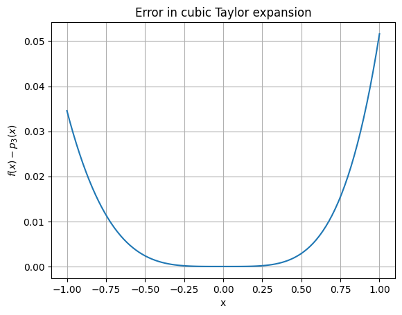
The remainder term does not give a sharp estimate. Plotting the error,

x = linspace(-1,1,100)
f = lambda x: exp(x)
p3 = lambda x: 1 + x + x**2/2 + x**3/6
e  = f(x) - p3(x)
print("Max error = ", abs(e).max())
plot(x,e)
title('Error in cubic Taylor expansion')
grid(True), xlabel('x'), ylabel('$f(x)-p_3(x)$');

Max error =  0.05161516179237857

we see that it is not uniformly distributed in the interval $[-1,1]$ . We have very good approximation near $x=0$ but poor approximation near the end-points of the interval.

7.3Cubic interpolation¶

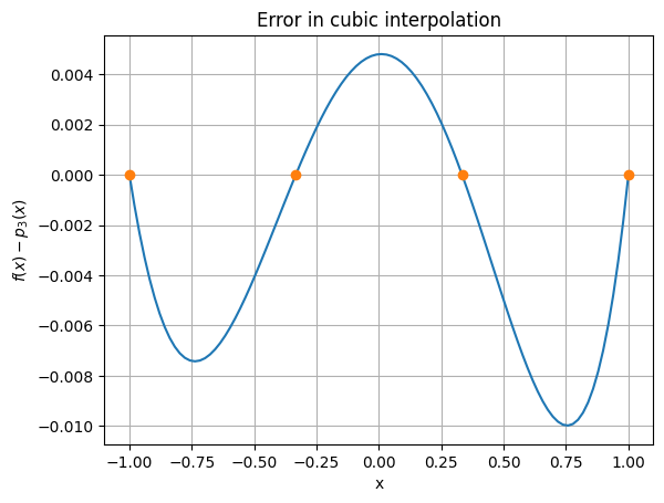
We can get much better cubic polynomial approximation than the Taylor polynomial. Let us interpolate a cubic polynomial at $\{-1, -\frac{1}{3}, +\frac{1}{3}, +1\}$ which yields

p_3(x) = 0.99519577 + 0.99904923 x + 0.54788486 x^2 + 0.17615196 x^3

(15)

The error in this approximation is shown below.

xi = linspace(-1,1,4)
yi = f(xi)
y  = barycentric_interpolate(xi,yi,x)
e  = f(x) - y
print("Max error = ",abs(e).max())
plot(x,e, xi, 0*xi, 'o')
title('Error in cubic interpolation')
grid(True), xlabel('x'), ylabel('$f(x)-p_3(x)$');

Max error =  0.009983970795226949

The maximum error is approximately 0.00998 which is almost five times smaller than the Taylor polynomial. The error is also more uniformly distributed and oscillates in sign.

References¶

Davis, P. J. (1963). Interpolation and Approximation. Dover Publications.

Numerical Analysis

Trigonometric interpolation