from pylab import *Consider the ODE system
The exact solution is
This solution is periodic. It also has a quadratic invariant
theta = linspace(0.0, 2*pi, 500)
xe = cos(theta)
ye = sin(theta)10.11.1Forward Euler scheme
def ForwardEuler(h,T):
    N = int(T/h)
    x,y = zeros(N),zeros(N)
    x[0] = 1.0
    y[0] = 0.0
    for n in range(1,N):
        x[n] = x[n-1] - h*y[n-1]
        y[n] = y[n-1] + h*x[n-1]
    return x,y
h = 0.02
T = 4.0*pi
x,y = ForwardEuler(h,T)
plot(xe,ye,'r--',label='Exact')
plot(x,y,label='FE')
legend()
grid(True)
gca().set_aspect('equal')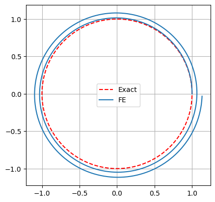
The phase space trajectory is spiralling outward.
10.11.2Backward Euler scheme
Eliminate from first equation and solve for to get
and now can also be computed.
def BackwardEuler(h,T):
    N = int(T/h)
    x,y = zeros(N),zeros(N)
    x[0] = 1.0
    y[0] = 0.0
    for n in range(1,N):
        x[n] = (x[n-1] - h*y[n-1])/(1.0 + h**2)
        y[n] = y[n-1] + h*x[n]
    return x,y
h = 0.02
T = 4.0*pi
x,y = BackwardEuler(h,T)
plot(xe,ye,'r--',label='Exact')
plot(x,y,label='BE')
legend()
grid(True)
gca().set_aspect('equal')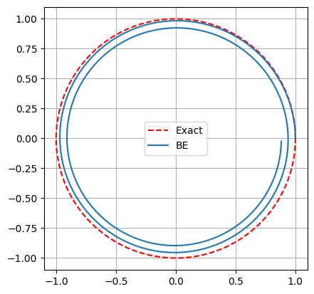
The phase space trajectory is spiralling inward.
10.11.3Trapezoidal scheme
Eliminate from first equation
and now can also be computed.
def Trapezoid(h,T):
    N = int(T/h)
    x,y = zeros(N),zeros(N)
    x[0] = 1.0
    y[0] = 0.0
    for n in range(1,N):
        x[n] = ((1.0-0.25*h**2)*x[n-1] - h*y[n-1])/(1.0 + 0.25*h**2)
        y[n] = y[n-1] + 0.5*h*(x[n-1] + x[n])
    return x,y
h = 0.02
T = 4.0*pi
x,y = Trapezoid(h,T)
plot(xe,ye,'r--',label='Exact')
plot(x,y,label='Trap')
legend()
grid(True)
gca().set_aspect('equal')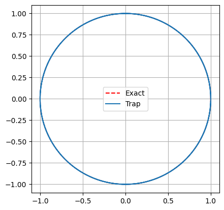
The phase space trajectory is exactly the unit circle.
Multiply first equation by and second equation by
Adding the two equations we get
Thus the Trapezoidal method is able to preserve the invariant.
10.11.4Partitioned Euler
This is a symplectic Runge-Kutta method. is updated explicitly and is updated implicitly.
The update of uses the latest updated value of .
def PartEuler(h,T):
    N = int(T/h)
    x,y = zeros(N),zeros(N)
    x[0] = 1.0
    y[0] = 0.0
    for n in range(1,N):
        x[n] = x[n-1] - h * y[n-1]
        y[n] = y[n-1] + h * x[n]
    return x,y
h = 0.02
T = 4.0*pi
x,y = PartEuler(h,T)
plot(xe,ye,'r--',label='Exact')
plot(x,y,label='PE')
legend()
grid(True)
gca().set_aspect('equal')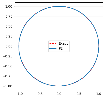
We get very good results, even though the method is only first order. We can also switch the implicit/explicit parts
10.11.5Classical RK4 scheme
def rhs(u):
    return array([u[1], -u[0]])

def RK4(h,T):
    N = int(T/h)
    u = zeros((N,2))
    u[0,0] = 1.0 # x
    u[0,1] = 0.0 # y
    for n in range(0,N-1):
        w = u[n,:]
        k0 = rhs(w)
        k1 = rhs(w + 0.5*h*k0)
        k2 = rhs(w + 0.5*h*k1)
        k3 = rhs(w + h*k2)
        u[n+1,:] = w + (h/6)*(k0 + k1 + k2 + k3)
    return u[:,0], u[:,1]
We test this method for a longer time.
h = 0.02
T = 10.0*pi
x,y = RK4(h,T)

plot(xe,ye,'r--',label='Exact')
plot(x,y,label='RK4')
legend()
grid(True)
gca().set_aspect('equal')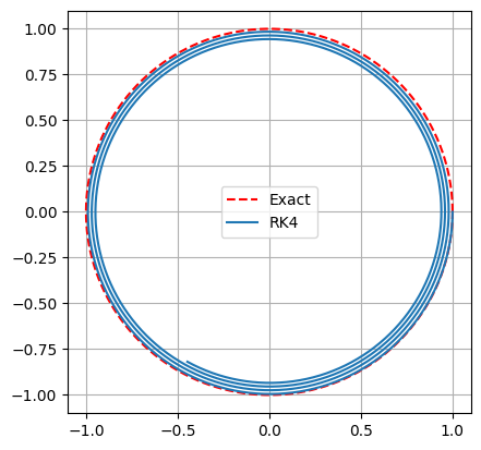
RK4 is a more accurate method compared to forward/backward Euler schemes, but it still loses total energy. The trajectory spirals inwards towards the origin.