Roots of polynomials - Numerical Analysis

#%config InlineBackend.figure_format = 'svg'
from pylab import *
import sympy

5.1Existence of roots¶

A polynomial of degree $n$ is a function of the form

p(x) = a_0 + a_1 x + a_2 x^2 + \ldots + a_n x^n, \qquad a_n \ne 0

(1)

where the coefficients $a_j$ may be real or complex.

If $r_1$ is a root of $p(x)$ , then it can be written as $p(x) = (x-r_1) q(x)$ where $q(x)$ is a polynomial of degree $n-1$ . Continuing this way, we see that $p(x)$ can be written as

p(x) = a_n (x-r_1) (x - r_2) \ldots (x - r_n)

(2)

Some of these roots may coincide; if $r_j$ appears $m$ times in the above factorization, then it is said to have multiplicity $m$ .

Note that we may not have any real roots even if all the coefficients are real, for example, $x^2+1=0$ has no real solutions.

5.2Roots from eigenvalues¶

Eigenvalues of a square matrix are the roots of a certain polynomial called the characteristic polynomial. Conversely, the roots of a given polynomial are the eigenvalues of a certain matrix.

The polynomial

p(x) = x^n + c_{n-1} x^{n-1} + \ldots + c_1 x + c_0

(3)

can be written as

p(x) = (-1)^n \det \begin{bmatrix} -x & & & & & -c_0 \\ 1 & -x & & & & -c_1 \\ & 1 & -x & & & -c_2 \\ & & 1 & \ddots & & \vdots \\ & & & \ddots & -x & -c_{n-2} \\ & & & & 1 & -x-c_{n-1} \\ \end{bmatrix}

(4)

with all other matrix entries being zero, i.e.,

p(x) = (-1)^n \det(A - xI), \qquad A = \begin{bmatrix} 0 & & & & & -c_0 \\ 1 & 0 & & & & -c_1 \\ & 1 & 0 & & & -c_2 \\ & & 1 & \ddots & & \vdots \\ & & & \ddots & 0 & -c_{n-2} \\ & & & & 1 & -c_{n-1} \\ \end{bmatrix}

(5)

Then

p(r) = 0 \limplies \det(A - rI) = 0

(6)

and every root of $p(x)$ is an eigenvalue of the $n \times n$ matrix $A$ , called the companion matrix. We have taken the coefficient of $x^n$ to be one but if this is not the case, then the coefficients can be scaled and this does not change the roots.

The next function computes the roots by finding eigenvalues, we do not assume that $a_n = 1$ , so we need to scale the coefficients.

# Input array a contains coefficient like this
#   p(x) = a[0] + a[1] * x + a[2] * x**2 + ... + a[n] * x**n
def roots1(a):
    n = len(a) - 1
    c = a[0:-1] / a[-1]
    A = zeros((n,n))
    A[:,-1] = -c
    A += diag(ones(n-1), -1)
    r = eigvals(A)
    return r

Make a polynomial of degree $n = m-1$ with random coefficients in $[-1,1]$ and find its roots.

m = 10
a = 2.0*rand(m) - 1.0
r = roots1(a)
print("roots = \n", r)

roots = 
 [-0.42792626+0.9554156j  -0.42792626-0.9554156j  -1.11699399+0.j
 -0.70192041+0.j          0.4352943 +0.58247496j  0.4352943 -0.58247496j
  0.92515954+0.39939538j  0.92515954-0.39939538j 10.92391124+0.j        ]

Check the roots by evaluating the polynomial at the roots. We use polyval which expects coefficients in opposite order to what we have assumed above.

print("|p(r)| = \n", abs(polyval(a[::-1],r)))

|p(r)| = 
 [3.68628542e-15 3.68628542e-15 9.21485110e-15 4.44089210e-16
 3.77442862e-15 3.77442862e-15 4.89953650e-16 4.89953650e-16
 6.08616218e-08]

These values are close to machine precision which can be considered to be zero.

The function numpy.roots computes roots by the same method.

r = roots(a[::-1])
print("roots = \n", r)

roots = 
 [10.92391124+0.j         -1.11699399+0.j         -0.42792626+0.9554156j
 -0.42792626-0.9554156j  -0.70192041+0.j          0.92515954+0.39939538j
  0.92515954-0.39939538j  0.4352943 +0.58247496j  0.4352943 -0.58247496j]

These roots are same as we got from our own function, but their ordering may be different.

Example 1

Consider the cubic polynomial

x^3 - 21 x^2 + 120 x - 100 = 0

(7)

whose exact roots are

x_1 = 1, \qquad x_2 = x_3 = 10

(8)

r = sympy.roots([1,-21,120,-100])
print('Roots = ',r)
for x in r:
    print(x)

Roots =  {1: 1, 10: 2}
1
10

Now let us perturb the highest coefficient by 1%

0.99 x^3 - 21 x^2 + 120 x - 100 = 0

(9)

The roots are now

x_1 \approx 1.000, \qquad x_2 \approx 11.17, \qquad x_3 \approx 9.041

(10)

r = sympy.roots([sympy.Integer(99)/100,-21,120,-100])
for x in r:
    print(sympy.N(x))

1.0001235059284 - 0.e-22*I

11.1706986297466 - 0.e-22*I
9.0412990764462 + 0.e-22*I

While $x_1$ changes by a small amount, the other two roots change by about 10% which is a large perturbation. Now change the coefficient to the other side by 1%.

1.01 x^3 - 21 x^2 + 120 x - 100 = 0

(11)

The roots are now

x_1 \approx 1.000, \qquad x_2, x_3 \approx 9.896 \pm 1.044 i

(12)

r = sympy.roots([sympy.Integer(101)/100,-21,120,-100])
for x in r:
    print(sympy.N(x))

0.999876592295142
9.89610130781283 - 1.04369535224477*I
9.89610130781283 + 1.04369535224477*I

Again, the double roots are very sensitive to perturbation of the coefficient. We say that the root finding problem is ill-conditioned.

5.3Test for ill-conditioning¶

Consider a polynomial

f(x) = a_n x^n + a_{n-1} x^{n-1} + \ldots + a_1 x + a_0

(13)

Let α be a single root, i.e., $f(\alpha) = 0$ and $f'(\alpha) \ne 0$ . Let us perturb the polynomial into a different polynomial

p(x) = f(x) + \epsilon g(x)

(14)

where

g(x) = b_n x^n + b_{n-1} x^{n-1} + \ldots + b_1 x + b_0

(15)

and let $\hat{\alpha} = \alpha + \delta$ be a root of $p(x)$ . Then, assuming the perturbation of the root is small, it can be estimated as

|\delta| \approx \left| \frac{\epsilon g(\alpha)}{f'(\alpha)} \right|

(16)

The change in the root is small, of $\order{\epsilon}$ ; however, depending on the value of the remaining factors in the above equation, the actual change can be larger than ε.

If α is a double root, then we can estimate the perturbation (Wilkinson)

|\delta| \approx \left[ - \frac{2\epsilon g(\alpha)}{f''(\alpha)} \right]^\half

(17)

Now, the change in the root is of $\order{\sqrt{\epsilon}}$ which is much larger than ε when $|\epsilon| \ll 1$ . Thus multiple roots can be expected to be very sensitive to changes in the coefficients.

Example 2

The polynomial

f(x) = x^3 - 21 x^2 + 120 x - 100

(18)

has roots $x_1 = 1$ , $x_2 = x_3 = 10$ . Let us perturb the highest power term, i.e., take $g(x) = x^3$ . Consider the single root $\alpha = x_1 = 1$ , $\epsilon = -0.01$ . Then

|\delta| \approx \left| \frac{(-0.01)(1)^3}{81} \right| \approx 0.0001

(19)

Hence the root $x_1$ is well-conditioned wrt perturbations in the coefficient $x^3$ . Now consider the double root $\alpha = x_2 = x_3 = 10$ . The perturbation in this root can be estimated as

|\delta| \approx \left| \frac{(-2)(-0.01)10^3}{18}\right|^\half \approx 1.054

(20)

This indicates that the double root is very sensitive to perturbation in the coefficient of $x^3$ , which we have observed in the previous example.

5.4Wilkinson’s polynomial¶

Wilkinson considered the following polynomial

p(x) = \prod_{i=1}^{20} (x - i), \qquad x \in [1,20]

(21)

We can find polynomial coefficients using sympy.

x, p = sympy.symbols('x p')
p = 1
for i in range(1,21):
    p = p * (x - i)
P = sympy.Poly(p, x)
a = P.coeffs()
for i,coef in enumerate(a):
    print("a[%2d] = %d" % (i,coef))

a[ 0] = 1
a[ 1] = -210
a[ 2] = 20615
a[ 3] = -1256850
a[ 4] = 53327946
a[ 5] = -1672280820
a[ 6] = 40171771630
a[ 7] = -756111184500
a[ 8] = 11310276995381
a[ 9] = -135585182899530
a[10] = 1307535010540395
a[11] = -10142299865511450
a[12] = 63030812099294896
a[13] = -311333643161390640
a[14] = 1206647803780373360
a[15] = -3599979517947607200
a[16] = 8037811822645051776
a[17] = -12870931245150988800
a[18] = 13803759753640704000
a[19] = -8752948036761600000
a[20] = 2432902008176640000

print('Monomial form = ', P)

Monomial form =  Poly(x**20 - 210*x**19 + 20615*x**18 - 1256850*x**17 + 53327946*x**16 - 1672280820*x**15 + 40171771630*x**14 - 756111184500*x**13 + 11310276995381*x**12 - 135585182899530*x**11 + 1307535010540395*x**10 - 10142299865511450*x**9 + 63030812099294896*x**8 - 311333643161390640*x**7 + 1206647803780373360*x**6 - 3599979517947607200*x**5 + 8037811822645051776*x**4 - 12870931245150988800*x**3 + 13803759753640704000*x**2 - 8752948036761600000*x + 2432902008176640000, x, domain='ZZ')

The coefficients are returned in this order

p(x) = a[0] x^{20} + a[1] x^{19} + \ldots + a[19] x + a[20]

(22)

i.e., a[0] is the coefficient of the largest degree term. We note that the coefficients are very large.

This function computes the polynomial in factored form.

# As a product of factors
def wpoly(x):
    p = 1.0
    for i in range(1,21):
        p = p * (x - i)
    return p

Plot the polynomial in $[1,20]$ by sampling it on a uniform grid using monomial form.

xp = linspace(1,20,1000)
yp = polyval(a,xp)
plot(xp,yp)
plot(arange(1,21),zeros(20),'o',label='Roots')
title("Monomial form")
legend(), grid(True), ylim(-1e13,1e13);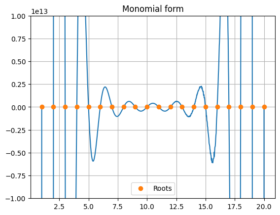

Computing the polynomial as a monomial is subject to lot of rounding errors since the coefficients are very large, see the jagged nature of the curve around $x=15$ . If we plot it in factored form, it does not suffer so much from rounding errors.

xp = linspace(1,20,1000)
yp = wpoly(xp)
plot(xp,yp)
plot(arange(1,21),zeros(20),'o',label='Roots')
title("Factored form")
legend(), grid(True), ylim(-1e13,1e13);

Find the roots using numpy.roots which computes it using the eigenvalue approach

r = roots(a)
print(r)

[19.99980929 19.00190982 17.99092135 17.02542715 15.94628672 15.0754938
 13.91475559 13.07431403 11.95328325 11.02502293  9.99041304  9.00291529
  7.99935583  7.000102    5.99998925  5.00000067  3.99999998  3.
  2.          1.        ]

The relative error in the roots is shown in the figure.

rexact = arange(20,0,-1)
semilogy(rexact, abs(r-rexact)/rexact, 'o')
xticks(rexact), grid(True), xlabel('Exact root'), ylabel('Relative error');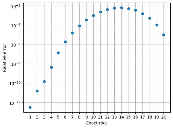

Randomly perturb the monomial coefficients and find roots

a_0(1 + \epsilon r_0) x^{20} + a_1 (1+ \epsilon r_1) x^{19} + \ldots + a_{20}(1+ \epsilon r_{20})

(23)

where $\epsilon = 10^{-10}$ and each $r_j$ is an independent Gaussian random variable with mean zero and standard deviation 1. We perform 100 random perturbations of the coefficients and plot the resulting roots on a single plot.

eps   = 1e-10 # Relative perturbation
nsamp = 100   # 100 random perturbations
for i in range(nsamp):
    r = normal(0.0, 1.0, 21)
    aa = a * (1 + eps * r)
    root = roots(aa)
    plot(real(root), imag(root),'k.')
plot(arange(1,21),zeros(20), 'ro')
xlabel('Real'); ylabel('Imag');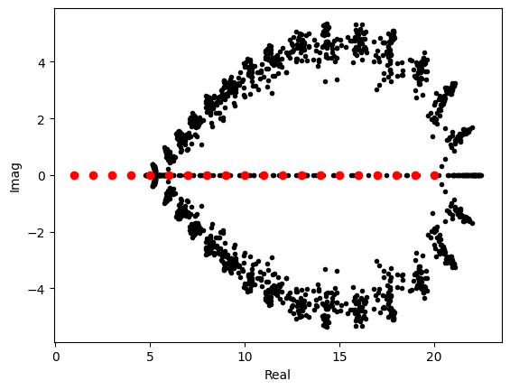

The relative perturbation in coefficients is $O(10^{-10})$ while the change in roots is $O(1)$ , which indicates a very high sensitivity wrt the coefficients. The roots 14,15,16 seem to experience the largest perturbation.

Using the estimate for root perturbation, we see that if the coefficient $a_i$ is changed to $a_i + \Delta a_i$ , the root $r_j$ changes to $\Delta r_j$ , and

\kappa(r_j, a_i) := \frac{ |\Delta r_j/r_j| }{ |\Delta a_i/a_i|} \approx \left| \frac{a_i r_j^{n-i}}{p'(r_j)|} \right|

(24)

is the condition number of $r_j$ wrt perturbations in $a_i$ . The condition number means

\kappa = \frac{\textrm{Relative change in output}}{\textrm{Relative change in input}}

(25)

A large value indicates high sensitity of the root (output) to changes in coefficients (input). The most sensitive root is $r=15$ wrt perturbations in $a_{5} \approx 1.67 \times 10^9$

\kappa(r=15, a_{5}) = \frac{1.67 \times 10^9 \cdot 15^{20-5}}{5! \cdot 14!} \approx 6.99 \times 10^{13}

(26)

References¶

Corless, R. M., & Sevyeri, L. R. (2020). The Runge Example for Interpolation and Wilkinson’s Examples for Rootfinding. SIAM Review, 62(1), 231–243. 10.1137/18M1181985
Trefethen, L. N. (2019). Approximation Theory and Approximation Practice, Extended Edition. Society for Industrial. 10.1137/1.9781611975949
Boyd, J. P. (2002). Computing Zeros on a Real Interval through Chebyshev Expansion and Polynomial Rootfinding. SIAM Journal on Numerical Analysis, 40(5), 1666–1682. 10.1137/S0036142901398325

Numerical Analysis

Homotopy and continuation methods