from pylab import *Consider the BVP
with boundary conditions
The exact solution is given by
10.13.1Finite difference method
Make a uniform grid of points such that
Then we approximate the differential equation by finite differences
with the boundary condition
This is a non-linear system of equations. We can eliminate and form a problem to find the remaining unknowns. Define
Then is a map from to . The Newton method is given by
The Jacobian is given by
and it is a tri-diagonal matrix, since depends only on .
def yexact(x):
    return 1.0/(exp(x)+exp(-x))

# Computes the vector phi(y): length (n-1)
# y = [y0, y1, ..., yn] = length n+1
def phi(y):
    n   = len(y) - 1
    h   = 2.0/n
    res = zeros(n-1)
    for i in range(1,n):
        dy = (y[i+1] - y[i-1])/(2.0*h)
        res[i-1] = (y[i-1] - 2.0*y[i] + y[i+1])/h**2 - 2.0*dy**2/y[i] + y[i]
    return res

# Computes Jacobian d(phi)/dy: (n-1)x(n-1)
# y = [y0, y1, ..., yn] = length n+1
def dphi(y):
    n   = len(y) - 1
    h   = 2.0/n
    res = zeros((n-1,n-1))
    for i in range(1,n):
        dy = (y[i+1] - y[i-1])/(2.0*h)
        if i > 1:
            res[i-1,i-2] = 1.0/h**2 + 4.0*dy/y[i]
        res[i-1,i-1] = -2.0/h**2 + 1.0 - 2.0*(dy/y[i])**2
        if i < n-1:
            res[i-1,i] = 1.0/h**2 - 4.0*dy/y[i]
    return res
We now solve the problem with Newton method.
n = 50

# Initial guess for y
y = zeros(n+1)
y[:] = 1.0/(exp(1) + exp(-1))

maxiter = 100
TOL = 1.0e-6
it = 0
while it < maxiter:
    b = -phi(y)
    if linalg.norm(b) < TOL:
        break
    A = dphi(y)
    v = linalg.solve(A,b)
    y[1:n] = y[1:n] + v
    it += 1
print("Number of iterations = %d" % it)
x = linspace(-1.0,1.0,n+1)
plot(x,y,'o',x,yexact(x))
legend(("Numerical","Exact"))
xlabel("x"), ylabel("y");
Number of iterations = 13
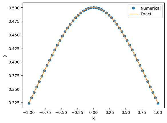
Note that y is initially filled with boundary condition and then we update only the other values y[1:n] with Newton method. Thus during the Newton updates, y always satisfies the boundary condition.