Asymptotic stability: Adams, BDF

See here for the schemes

For stability we require the roots $w$ of

\rho(w) - z \sigma(w)

(1)

to be less than one

|w_i(z)| < 1

(2)

We find the values of $z$ for which $|w|=1$

w = e^{i \theta}, \qquad z = \frac{\rho(e^{i\theta})}{\sigma(e^{i\theta})}

(3)

import numpy as np
from matplotlib import pyplot as plt

def AB2(theta):
    w = np.exp(1j*theta)
    return (w**2 - w)/(3.0*w/2.0 - 1.0/2.0)

def AB3(theta):
    w = np.exp(1j*theta)
    return (w**3 - w**2)/(23.0*w**2/12.0 - 4.0*w/3.0 + 5.0/12.0)

theta = np.linspace(0,2*np.pi,1000)

z = AB2(theta)
plt.plot(np.real(z),np.imag(z))

z = AB3(theta)
plt.plot(np.real(z),np.imag(z))

plt.legend(("AB2","AB3"))
plt.grid(True)
plt.xlim([-2, 1])
plt.ylim([-1, 1])
plt.axis('equal');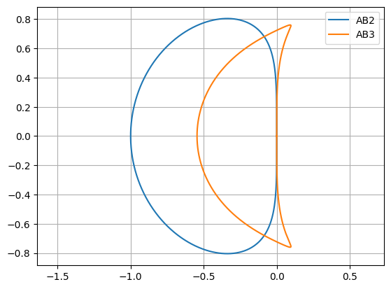

def AM2(theta):
    w = np.exp(1j*theta)
    return (w**2 - w)/(5.0*w**2/12.0 + 2.0*w/3.0 - 1.0/12.0)

def AM3(theta):
    w = np.exp(1j*theta)
    return (w**3 - w**2)/(3.0*w**3/8.0 + 19.0*w**2/24.0 - 5.0*w/24.0 - 1.0/24.0)

z = AM2(theta)
plt.plot(np.real(z),np.imag(z))

z = AM3(theta)
plt.plot(np.real(z),np.imag(z))

plt.legend(("AM2","AM3"))
plt.xlim([-7, 2])
plt.ylim([-4, 4])
plt.grid(True)
plt.axis('equal');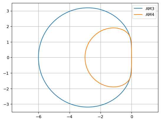

These discs are bigger than those for the AB methods, but they are also not A-stable methods.

Stability domains for Backward Differentiation Formula¶

See here for the schemes

Backward differentiation formula

def BDF1(theta):
    w = np.exp(1j*theta)
    return (w-1)/w

def BDF2(theta):
    w = np.exp(1j*theta)
    return (w**2 - 4.0*w/3.0 + 1.0/3.0)/(2.0*w**2/3.0)

def BDF3(theta):
    w = np.exp(1j*theta)
    return (w**3 - 18.0*w**2/11.0 + 9.0*w/11.0 - 2.0/11.0)/(6.0*w**3/11.0)

def BDF4(theta):
    w = np.exp(1j*theta)
    return (w**4 - 48.0*w**3/25.0 + 36.0*w**2/25.0 - 16.0*w/25.0 + 3.0/25.0)/(12.0*w**4/25.0)

z = BDF1(theta)
plt.plot(np.real(z),np.imag(z))

z = BDF2(theta)
plt.plot(np.real(z),np.imag(z))

z = BDF3(theta)
plt.plot(np.real(z),np.imag(z))

z = BDF4(theta)
plt.plot(np.real(z),np.imag(z))

plt.legend(("BDF1","BDF2","BDF3","BDF4"))
plt.xlim([-1, 18])
plt.ylim([-8, 8])
plt.grid(True)
plt.axis('equal');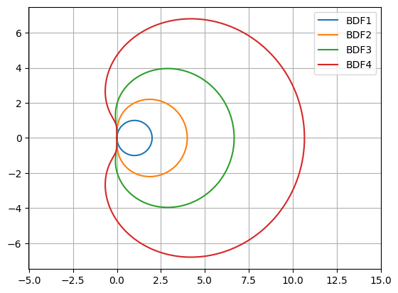

The region of asymptotic stability is the exterior of these discs. Only the BDF1 and BDF2 discs are entirely to the right of the imaginary axis and these are A-stable.