1 Single interval ¶ Trapezoidal method used a linear approximation to estimate the integral.
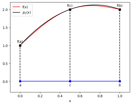
To improve the accuracy, let us use a quadratic approximation. For the
function f : [ a , b ] → R f : [a,b] \to \re f : [ a , b ] → R , we first construct a quadratic polynomial
p 2 ( x ) p_2(x) p 2 ( x ) that interpolates at a , b , c = 1 2 ( a + b ) a, b, c = \half(a+b) a , b , c = 2 1 ( a + b )
p 2 ( a ) = f ( a ) , p 2 ( b ) = f ( b ) , p 2 ( c ) = f ( c ) p_2(a) = f(a), \qquad p_2(b) = f(b), \qquad p_2(c) = f(c) p 2 ( a ) = f ( a ) , p 2 ( b ) = f ( b ) , p 2 ( c ) = f ( c ) and the
approximation to the integral is
I 2 ( f ) = ∫ a b p 2 ( x ) d x = h 3 [ f ( a ) + 4 f ( c ) + f ( b ) ] , h = 1 2 ( b − a ) I_2(f) = \int_a^b p_2(x) \ud x = \frac{h}{3}[f(a) + 4 f(c) + f(b)], \qquad h = \half(b-a) I 2 ( f ) = ∫ a b p 2 ( x ) d x = 3 h [ f ( a ) + 4 f ( c ) + f ( b )] , h = 2 1 ( b − a ) This is called Simpson rule. The error is
E 2 ( f ) = I ( f ) − I 2 ( f ) = ∫ a b ( x − a ) ( x − c ) ( x − b ) ⏟ changes sign at x = c f [ a , b , c , x ] d x E_2(f) = I(f) - I_2(f) = \int_a^b \underbrace{(x-a)(x-c)(x-b)}_{\textrm{changes sign at $x=c$}} f[a,b,c,x] \ud x E 2 ( f ) = I ( f ) − I 2 ( f ) = ∫ a b changes sign at x = c ( x − a ) ( x − c ) ( x − b ) f [ a , b , c , x ] d x Define
w ( x ) = ∫ a x ( t − a ) ( t − c ) ( t − b ) d x w(x) = \int_a^x (t-a)(t-c)(t-b)\ud x w ( x ) = ∫ a x ( t − a ) ( t − c ) ( t − b ) d x Then
w ( a ) = w ( b ) = 0 , w ( x ) > 0 ∀ x ∈ ( a , b ) w(a) = w(b) = 0, \qquad w(x) > 0 \quad \forall x \in (a,b) w ( a ) = w ( b ) = 0 , w ( x ) > 0 ∀ x ∈ ( a , b ) and
w ′ ( x ) = ( x − a ) ( x − c ) ( x − b ) w'(x) = (x-a)(x-c)(x-b) w ′ ( x ) = ( x − a ) ( x − c ) ( x − b ) Hence the error can be written as
E 2 ( f ) = ∫ a b w ′ ( x ) f [ a , b , c , x ] d x = [ w ( x ) f [ a , b , c , x ] ] a b − ∫ a b w ( x ) d d x f [ a , b , c , x ] d x = − ∫ a b w ( x ) f [ a , b , c , x , x ] d x \begin{aligned}
E_2(f)
&= \int_a^b w'(x) f[a,b,c,x] \ud x \\
&= [w(x) f[a,b,c,x]]_a^b - \int_a^b w(x) \dd{}{x} f[a,b,c,x] \ud x \\
&= - \int_a^b w(x) f[a,b,c,x,x] \ud x
\end{aligned} E 2 ( f ) = ∫ a b w ′ ( x ) f [ a , b , c , x ] d x = [ w ( x ) f [ a , b , c , x ] ] a b − ∫ a b w ( x ) d x d f [ a , b , c , x ] d x = − ∫ a b w ( x ) f [ a , b , c , x , x ] d x Now we can apply the integral mean value theorem
E 2 ( f ) = − f [ a , b , c , ξ , ξ ] ∫ a b w ( x ) d x , for some ξ ∈ [ a , b ] = − 1 24 f ( 4 ) ( η ) [ 4 15 h 5 ] , for some η ∈ [ a , b ] \begin{aligned}
E_2(f)
&= -f[a,b,c,\xi,\xi] \int_a^b w(x) \ud x, \quad \textrm{for some $\xi \in [a,b]$} \\
&= -\frac{1}{24} f^{(4)}(\eta) \left[ \frac{4}{15} h^5 \right], \quad \textrm{for some $\eta \in [a,b]$}
\end{aligned} E 2 ( f ) = − f [ a , b , c , ξ , ξ ] ∫ a b w ( x ) d x , for some ξ ∈ [ a , b ] = − 24 1 f ( 4 ) ( η ) [ 15 4 h 5 ] , for some η ∈ [ a , b ] The error in Simpson rule is given by
E 3 ( f ) = − 1 90 h 5 f ( 4 ) ( η ) , for some η ∈ [ a , b ] E_3(f) = -\frac{1}{90} h^5 f^{(4)}(\eta), \quad \textrm{for some $\eta \in [a,b]$} E 3 ( f ) = − 90 1 h 5 f ( 4 ) ( η ) , for some η ∈ [ a , b ] By construction, Simpson rule is exact for quadratic polynomials. The
error formula tells us that even for cubic polynomials, the error is
zero.
2 Composite Simpson rule ¶ Let n ≥ 2 n \ge 2 n ≥ 2 be even, the spacing between points h = ( b − a ) / n h = (b-a)/n h = ( b − a ) / n and the
n + 1 n+1 n + 1 points
x j = a + j h , j = 0 , 1 , 2 , … , n x_j = a + j h, \quad j=0,1,2,\ldots,n x j = a + jh , j = 0 , 1 , 2 , … , n Then
I ( f ) = ∫ a b f ( x ) d x = ∑ j = 1 n / 2 ∫ x 2 j − 2 x 2 j f ( x ) d x = ∑ j = 1 n / 2 { h 3 [ f 2 j − 2 + 4 f 2 j − 1 + f 2 j ] − h 5 90 f ( 4 ) ( η j ) } , η j ∈ [ x 2 j − 2 , x 2 j ] \begin{aligned}
I(f)
&= \int_a^b f(x) \ud x \\
&= \sum_{j=1}^{n/2} \int_{x_{2j-2}}^{x_{2j}} f(x) \ud x \\
&= \sum_{j=1}^{n/2}\left\{ \frac{h}{3}[f_{2j-2} + 4 f_{2j-1} + f_{2j}] - \frac{h^5}{90} f^{(4)}(\eta_j) \right\}, \quad \eta_j \in [x_{2j-2},x_{2j}]
\end{aligned} I ( f ) = ∫ a b f ( x ) d x = j = 1 ∑ n /2 ∫ x 2 j − 2 x 2 j f ( x ) d x = j = 1 ∑ n /2 { 3 h [ f 2 j − 2 + 4 f 2 j − 1 + f 2 j ] − 90 h 5 f ( 4 ) ( η j ) } , η j ∈ [ x 2 j − 2 , x 2 j ] The composite Simpson rule is
I n ( f ) = h 3 [ f 0 + 4 f 1 + 2 f 2 + … + 2 f n − 2 + 4 f n − 1 + f n ] I_n(f) = \frac{h}{3}[ f_0 + 4 f_1 + 2 f_2 + \ldots + 2 f_{n-2} + 4 f_{n-1} + f_n] I n ( f ) = 3 h [ f 0 + 4 f 1 + 2 f 2 + … + 2 f n − 2 + 4 f n − 1 + f n ] The error in this approximation is
E n ( f ) = I ( f ) − I n ( f ) = − h 5 90 ( n 2 ) [ 2 n ∑ j = 1 n / 2 f ( 4 ) ( η j ) ] E_n(f) = I(f) - I_n(f) = -\frac{h^5}{90} \left(\frac{n}{2}\right) \left[ \frac{2}{n} \sum_{j=1}^{n/2} f^{(4)}(\eta_j) \right] E n ( f ) = I ( f ) − I n ( f ) = − 90 h 5 ( 2 n ) ⎣ ⎡ n 2 j = 1 ∑ n /2 f ( 4 ) ( η j ) ⎦ ⎤ If the fourth derivative is continuous, then
E n ( f ) = − 1 180 ( b − a ) h 4 f ( 4 ) ( η ) , for some η ∈ [ a , b ] E_n(f) = -\frac{1}{180} (b-a)h^4 f^{(4)}(\eta), \quad \textrm{for some $\eta \in [a,b]$} E n ( f ) = − 180 1 ( b − a ) h 4 f ( 4 ) ( η ) , for some η ∈ [ a , b ] We can also derive the asymptotic error formula
E n ( f ) ≈ E ~ n ( f ) = − h 4 180 [ f ( 3 ) ( b ) − f ( 3 ) ( a ) ] E_n(f) \approx \tilde E_n(f) = -\frac{h^4}{180}[ f^{(3)}(b) - f^{(3)}(a)] E n ( f ) ≈ E ~ n ( f ) = − 180 h 4 [ f ( 3 ) ( b ) − f ( 3 ) ( a )] def simpson(a,b,n,f,df3):
h = (b-a)/n
x = linspace(a,b,n+1)
y = f(x)
res = 4.0*sum(y[1:n:2]) + 2.0*sum(y[2:n-1:2]) + y[0] + y[n]
est = -(h**4/180.0)*(df3(b) - df3(a))
return (h/3.0)*res, est
3 Compare Trapezoid and Simpson ¶ The next function implements Trapezoid and Simpson methods.
# Performs Trapezoid and Simpson quadrature
def integrate(a,b,n,f):
h = (b-a)/n
x = linspace(a,b,n+1)
y = f(x)
res1 = 0.5*y[0] + sum(y[1:n]) + 0.5*y[n]
res2 = 4.0*sum(y[1:n:2]) + 2.0*sum(y[2:n-1:2]) + y[0] + y[n]
return h*res1, (h/3.0)*res2
The next function performs convergence test.
def test(a,b,f,Ie,n,N):
e1,e2 = zeros(N), zeros(N)
for i in range(N):
I1,I2 = integrate(a,b,n,f)
e1[i],e2[i] = Ie - I1, Ie - I2
if i > 0:
print('%6d %18.8e %14.5g %18.8e %14.5g'%
(n,e1[i],e1[i-1]/e1[i],e2[i],e2[i-1]/e2[i]))
else:
print('%6d %18.8e %14.5g %18.8e %14.5g'%(n,e1[i],0,e2[i],0))
n = 2*n