Barycentric form - Numerical Analysis

#%config InlineBackend.figure_format = 'svg'
from pylab import *

The Lagrange interpolation polynomial of degree $N$ is

p(x) = \sum_{j=0}^N f(x_j) \ell_j(x) \qquad \textrm{where} \qquad \ell_j(x) = \frac{\prod\limits_{i=0,i\ne j}^N (x-x_i)}{\prod\limits_{i=0,i \ne j}^N(x_j - x_i)}

(1)

There are some issues in computing it as written above.

The denominators in $\ell_j$ do not depend on $x$ and can be pre-computed and stored. Then for every $x$ , the evaluation of $p(x)$ requires $O(N^2)$ flops. Ideally, we desire a method which takes $O(N)$ flops.
Also, if we add a new data pair $(x_{N+1},f_{N+1})$ , then this requires a new computation from scratch.
Moreover, the numerical evaluation is also unstable to round-off errors (See page 51 in Powell, Approximation theory and methods, 1981.)

These problems can be overcome by using alternate forms of Lagrange interpolation Berrut & Trefethen, 2004, Trefethen, 2019.

7.3.1Improved Lagrange formula¶

Define

\begin{gather} \ell(x) = \omega_N(x) = (x-x_0)(x-x_1) \ldots (x-x_N) \\ w_j = \frac{1}{\prod\limits_{k=0, k \ne j}^N (x_j - x_k)} = \frac{1}{\ell'(x_j)}, \qquad j=0,1,\ldots,N \end{gather}

(2)

The Lagrange polynomials can be written as

\ell_j(x) = \frac{\ell(x)}{\ell'(x_j) (x - x_j)} = \ell(x) \frac{w_j}{x-x_j}

(3)

and the interpolant is given by

p(x) = \ell(x) \sum_{j=0}^N \frac{w_j}{x-x_j} f_j

(4)

This is called the first form of barycentric interpolation formula and is due to Rutishauser. For each $x$

calculation of $\{w_j\}$ requires $O(N^2)$ flops, and these are independent of $x$
calculation of $\ell(x)$ requires $O(N)$ flops
calculation of the other term requires $O(N)$ flops

so the complexity of this formula is $O(N)$ . Once the weights $w_j$ are known, this permits interpolation of as many functions as desired in $O(N)$ operations. If a new data point $(x_{N+1},f_{N+1})$ is added

Divide each $w_j$ by $(x_j - x_{N+1})$ which needs $O(N+1)$ flops
compute $w_{N+1}$ at $O(N+1)$ flops

The total cost of updating the formula is $O(N)$ flops.

7.3.2Barycentric formula¶

Since $\ell_j$ form a partition of unity

1 = \sum_{j=0}^N \ell_j(x) = \ell(x) \sum_{j=0}^N \frac{w_j}{x-x_j} \limplies \ell(x) = \frac{ 1 }{ \sum_{j=0}^N \frac{w_j}{x- x_j} }

(6)

the interpolant can be written as

p(x) = \frac{ \sum_{j=0}^N \frac{w_j}{x-x_j} f_j }{ \sum_{j=0}^N \frac{w_j}{x- x_j} }

(7)

which is called the second form of barycentric formula. This has same complexity as the previous form. Higham, 2004 has shown that barycentric formula is numerically stable. This form is general since it takes any node sets and computes the weights.

7.3.3Weights¶

For special node distributions, we can simplify the weight calculation and obtain explicit expressions, as shown in the next sections.

7.3.3.1Equispaced points¶

If we have $N+1$ equispaced data points in $[-1,+1]$ , with spacing $h = \frac{2}{N}$ , the weights are given by

w_j = (-1)^{N-j} \binom{N}{j} \frac{1}{h^n n!}

(8)

Since the weights appear both in numerator and denominator, we can remove any factor independent of $j$ and use

w_j = (-1)^{j} \binom{N}{j}

(9)

If the interval is $[a,b]$ , we have to multiply the above $w_j$ by $2^N (b-a)^{-N}$ , but this factor can also be dropped since it is common to numerator and denominator. The weights $w_j$ change by exponentially large factors,

\frac{\max_j |w_j|}{\min_j |w_j|} \approx 2^N

(10)

This leads to ill-conditioning and Runge phenomenon. This is not a consequence of the barycentric formula, but is intrinsic to interpolation using equispaced data.

7.3.3.2Chebyshev points of first kind¶

The points and weights are given by

x_j = \cos\left( \frac{2j+1}{2N+2} \pi \right), \quad w_j = (-1)^j \sin\left( \frac{2j+1} {2N+2} \pi \right), \quad j=0,1,\ldots,N

(11)

These weights vary by factors of $O(N)$ , since

\frac{\max_j |w_j|}{\min_j |w_j|} \approx \frac{ \sin\left( \frac{2(N/2)+1}{2N+2} \pi \right) } { \sin\left( \frac{2(0)+1}{2N+2} \pi \right)} \approx \frac{\sin(\half\pi)}{\frac{\pi} {2N+2}} = O(N) \quad \textrm{for large $N$}

(12)

not exponentially as in case of uniformly spaced points. The weights can be computed in $O(N)$ operations.

7.3.3.3Chebyshev points of second kind¶

The points are given by

x_i = \cos\left( \frac{N-i}{N} \pi \right), \qquad i=0,1,2,\ldots,N

(13)

and the weights are

w_0 = \half, \qquad w_i = (-1)^i, \quad i=1,2,\ldots,N-1, \qquad w_N = \half (-1)^N

(14)

Example 1

Let us interpolate the Runge function on $[-1,+1]$

f(x) = \frac{1}{1 + 16 x^2}

(15)

using the Barycentric formula

p(x) = \frac{ \sum_{i=0}^N \frac{w_i}{x - x_i} f_i }{ \sum_{i=0}^N \frac{w_i}{x - x_i} }

(16)

where the weight $w_i$ is given by

w_i = \frac{1}{\prod_{j=0,j\ne i}^N (x_i - x_j)}

(17)

This is the function we want to interpolate.

def fun(x):
    f = 1.0/(1.0+16.0*x**2)
    return f

We next write a function that constructs and evaluates the Lagrange interpolation.

# X[nX], Y[nX] : Data points
# x[nx]        : points where we want to evaluate
def BaryInterp(X,Y,x):
    nx = len(x)
    nX = len(X)
    # compute the weights
    w = ones(nX)
    for i in range(nX):
        for j in range(nX):
            if i != j:
                w[i] = w[i]/(X[i]-X[j])
    # Evaluate the polynomial at x
    f = empty_like(x)
    for i in range(nx):
        num, den = 0.0, 0.0
        for j in range(nX):
            if abs(x[i]-X[j]) < 1.0e-15:
                num = Y[j]
                den = 1.0
                break
            else:
                num += Y[j]*w[j]/((x[i]-X[j]))
                den += w[j]/(x[i]-X[j])
        f[i] = num/den
    return f

xmin, xmax = -1.0, +1.0
N = 15 # Degree of polynomial

We first interpolate on uniformly spaced points.

X = linspace(xmin,xmax,N+1)
Y = fun(X)
x = linspace(xmin,xmax,100)
fi = BaryInterp(X,Y,x)
fe = fun(x)
plot(x,fe,'b--',x,fi,'r-',X,Y,'o')
title('Degree '+str(N)+' using uniform points')
legend(("True function","Interpolation","Data"),loc='lower center');

Next, we interpolate on Chebyshev points.

X = cos(linspace(0.0,pi,N+1))
Y = fun(X)
x = linspace(xmin,xmax,100)
fi = BaryInterp(X,Y,x)
fe = fun(x)
plot(x,fe,'b--',x,fi,'r-',X,Y,'o')
title('Degree '+str(N)+' using Chebyshev points')
legend(("True function","Interpolation","Data"),loc='upper right');

Example 2 (Barycentric Lagrange interpolation on Chebyshev points)

Let us interpolate the Runge function on $[-1,+1]$

f(x) = \frac{1}{1 + 16 x^2}

(18)

using the Barycentric formula

p(x) = \frac{ \sum\limits_{i=0}^N{}' \frac{(-1)^i}{x - x_i} f_i }{ \sum\limits_{i=0}^N{}' \frac{(-1)^i}{x - x_i} }

(19)

where the prime on the summation means that the first and last terms must be multiplied by a factor of half.

The next function evaluates the Lagrange interpolation using Chebyshev points.

def BaryChebInterp(X,Y,x):
    nx = len(x)
    nX = len(X)
    # Compute weights
    w       = (-1.0)**arange(0,nX)
    w[0]    = 0.5*w[0]
    w[nX-1] = 0.5*w[nX-1]
    # Evaluate barycentric foruma at x values
    f = empty_like(x)
    for i in range(nx):
        num, den = 0.0, 0.0
        for j in range(nX):
            if abs(x[i]-X[j]) < 1.0e-15:
                num = Y[j]
                den = 1.0
                break
            else:
                num += Y[j]*w[j]/((x[i]-X[j]))
                den += w[j]/(x[i]-X[j])
        f[i] = num/den
    return f

Define the function to be interpolated.

xmin, xmax = -1.0, +1.0
f = lambda x: 1.0/(1.0+16.0*x**2)

Let us interpolate on Chebyshev points.

N = 19 # degree of polynomial
X = cos(linspace(0.0,pi,N+1))
Y = fun(X)
x = linspace(xmin,xmax,100)
fi = BaryChebInterp(X,Y,x)
fe = fun(x)
figure(figsize=(8,5))
plot(x,fe,'b--',x,fi,'r-',X,Y,'o')
title("Chebshev interpolation, degree = " + str(N))
legend(("True function","Interpolation","Data"),loc='upper right')
xlabel('x'), ylabel('f(x)')
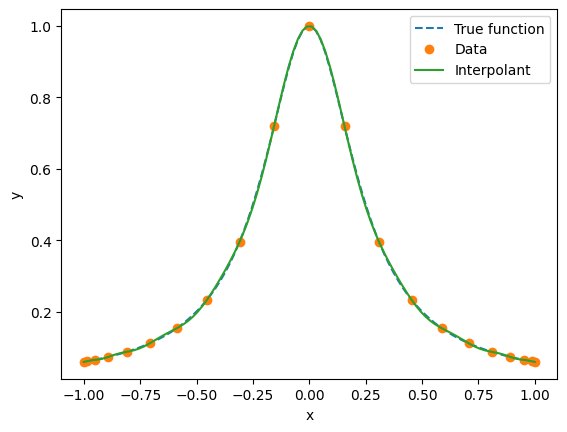
axis([-1.0,+1.0,0.0,1.1]);

7.3.4Using `scipy.interpolate`¶

scipy.interpolate provides many methods for polynomial interpolation, including barycentric form.

fun = lambda x: 1.0/(1.0 + 16.0 * x**2)
N   = 20
xi  = cos(linspace(0.0,pi,N+1))
yi  = fun(xi)
x   = linspace(xmin,xmax,100)

Using scipy.interpolate.barycentric_interpolate

from scipy.interpolate import barycentric_interpolate
y = barycentric_interpolate(xi, yi, x)
plot(x,  fun(x), '--', label='True function')
plot(xi, yi,     'o',  label='Data')
plot(x,  y,      '-',  label='Interpolant')
legend(), xlabel('x'), ylabel('y'), title('Degree = '+str(N));

Using scipy.interpolate.BarycentricInterpolater

from scipy.interpolate import BarycentricInterpolator
P = BarycentricInterpolator(xi, yi)
plot(x,  fun(x), '--', label='True function')
plot(xi, yi,     'o',  label='Data')
plot(x,  P(x),   '-',  label='Interpolant')
legend(), xlabel('x'), ylabel('y');

The second form is useful to construct a representation of the interpolant once, and repeatedly use it to evaluate at different values of $x$ .

Example 3

Interpolate $f(x) = \cos(4 \pi x)$ for $x \in [-1,1]$ for high degrees using uniform and Chebyshev points.

f  = lambda x: cos(4*pi*x)
xe = linspace(-1,1,1000)

figure(figsize=(10,10))
N = 20
for i in range(5):
    x1 = linspace(-1,1,N+1)
    y1 = f(x1)
    x2 = cos(linspace(0,pi,N+1))
    y2 = f(x2)
    y1e = barycentric_interpolate(x1,y1,xe)
    y2e = barycentric_interpolate(x2,y2,xe)
    err1 = abs(y1e - f(xe)).max()
    err2 = abs(y2e - f(xe)).max()
    print("N, Error = %3d %12.4e %12.4e" % (N,err1,err2))
    subplot(5,2,2*i+1)
    plot(xe,y1e), plot(xe,f(xe))
    text(0,0,'N='+str(N),ha='center',va='center')
    subplot(5,2,2*i+2)
    plot(xe,y2e), plot(xe,f(xe))
    text(0,0,'N='+str(N),ha='center')
    N = N + 10

N, Error =  20   7.6371e-02   2.1871e-04
N, Error =  30   1.7981e-06   1.5623e-10

N, Error =  40   7.3791e-07   1.7104e-15
N, Error =  50   3.2039e-04   1.7764e-15
N, Error =  60   4.8051e-01   1.7486e-15

This function is analytic in the complex plane, so uniform interpolation should also converge. The error decreases initially but starts to rise for higher degress. This is due to large round-off errors because the barycentric weights are large. Chebyshev points do not have this problem.

References¶

Berrut, J.-P., & Trefethen, L. N. (2004). Barycentric Lagrange Interpolation. SIAM Review, 46(3), 501–517. 10.1137/S0036144502417715
Trefethen, L. N. (2019). Approximation Theory and Approximation Practice, Extended Edition. Society for Industrial. 10.1137/1.9781611975949
Higham, N. J. (2004). The numerical stability of barycentric Lagrange interpolation. IMA Journal of Numerical Analysis, 24(4), 547–556. 10.1093/imanum/24.4.547

Numerical Analysis

Interpolation using polynomials