Interpolation using polynomials - Numerical Analysis

#%config InlineBackend.figure_format = 'svg'
from pylab import *
from scipy.interpolate import barycentric_interpolate

Polynomials are easy to evluate since they require only basic arithmetic operations: $-,+,\div$ . They can provide a good approximation to continuous functions as shown by Weirstrass Theorem.

6.2.1Interpolation using monomials¶

Given $N+1$ data

(x_i, y_i), \quad i=0,1,\ldots,N \qquad \textrm{with} \qquad y_i = f(x_i)

(1)

we can try to find a polynomial of degree $N$

p(x) = a_0 + a_1 x + \ldots + a_N x^N

(2)

that satisfies the interpolation conditions

p(x_i) = y_i, \qquad i=0,1,\ldots, N

(3)

This is a linear system of $N+1$ equations that can be written in matrix form

\underbrace{\begin{bmatrix} 1 & x_0 & x_0^2 & \ldots & x_0^N \\ 1 & x_1 & x_1^2 & \ldots & x_1^N \\ \vdots & \vdots & \ldots & \vdots \\ 1 & x_N & x_N^2 & \ldots & x_N^N \end{bmatrix}}_{V} \begin{bmatrix} a_0 \\ a_1 \\ \vdots \\ a_N \end{bmatrix} = \begin{bmatrix} y_0 \\ y_1 \\ \vdots \\ y_N \end{bmatrix}

(4)

This has a unique solution if the Vandermonde matrix $V$ is non-singular. Since

\det V = \prod_{j=0}^N \prod_{k=j+1}^N (x_k - x_j)

(5)

we can solve the problem provided the points $\{ x_i \}$ are distinct.

$V$ is non-singular. We can show this without computing the determinant. Assume that the $\{ x_i \}$ are distinct. It is enough to show that the only solution of $Va=0$ is $a=0$ . Note that the set of $N+1$ equations $Va=0$ is of the form

p(x_i) = 0, \qquad i=0,1,\ldots,N

(6)

which implies that $p(x)$ has $N+1$ distinct roots. But since $p$ is a polynomial of degree $N$ , this implies that $p(x) \equiv 0$ and hence each $a_i = 0$ ; the matrix $V$ is non-singular.

6.2.1.1Condition number of $V$ ¶

If we want to solve the interpolation problem by solving the matrix problem, then the condition number of the matrix becomes important. The condition number of a square matrix wrt some matrix norm is defined as

\kappa(A) = \norm{A} \cdot \norm{A^{-1}}

(7)

Matrices with large condition numbers cannot be solved accurately on a computer by Gaussian elimination due to possible growth of round-off errors.

Example 1

Take $(x_0,x_1,x_2) = (100,101,102)$ , then with $p(x) = a_0 + a_1 x + a_2 x^2$

V = \begin{bmatrix} 1 & 100 & 10000 \\ 1 & 101 & 10201 \\ 1 & 102 & 10402 \end{bmatrix}, \qquad \cond(V) \approx 10^8

(8)

If we scale the $x$ as $x \to \frac{x}{x_0}$ , then with $p(x) = a_0 + a_1 (x/x_0) + a_2 (x/x_0)^2$

\tilde{V} = \begin{bmatrix} 1 & 1.00 & 1.0000 \\ 1 & 1.01 & 1.0201 \\ 1 & 1.02 & 1.0402 \end{bmatrix}, \qquad \cond(\tilde{V}) \approx 10^5

(9)

Or we can shift the origin to $x_0$ , then with $p(x) = a_0 + a_1 (x-x_0) + a_2 (x-x_0)^2$

\hat{V} = \begin{bmatrix} 1 & 0 & 0 \\ 1 & 1 & 1 \\ 1 & 2 & 4 \end{bmatrix}, \qquad \cond(\hat{V}) \approx 14

(10)

The condition number can be improved by scaling and/or shifting the variables.

Remark 1

It is usually better to map the data to the interval $[-1,+1]$ or $[0,1]$ and then solve the interpolation problem on the mapped interval. Assuming that $x_0 < x_1 < \ldots x_N$ , define

\xi = \frac{x - x_0}{x_N - x_0}

(11)

and find a polynomial of the form

p(\xi) = a_0 + a_1 \xi + \ldots + a_N \xi^N

(12)

But still the condition number increases rapidly with $N$ . For $N=20$ we have a condition number of $8 \times 10^8$ even when using the interval $[-1,+1]$ .

We will use the numpy.linalg.cond function to compute the condition number. By default, it uses the 2-norm.

Nvalues, Cvalues = [], []
for N in range(1,30):
    x = linspace(-1.0,+1.0,N+1)
    V = zeros((N+1,N+1))
    for j in range(0,N+1):
        V[:,j] = x**j
    Nvalues.append(N), Cvalues.append(cond(V))
semilogy(Nvalues, Cvalues, 'o-')
xlabel('N'), ylabel('cond(V)'), grid(True);

The condition number is large for even moderate value of $N=30$ .

6.2.2Interpolating polynomials¶

6.2.3Lagrange interpolation¶

Lagrange interpolation provides the solution without having to solve a matrix problem. Define

\pi_i(x) = (x-x_0) \ldots (x-x_{i-1})(x-x_{i+1})\ldots (x-x_N)

(15)

and

\ell_i(x) = \frac{\pi_i(x)}{\pi_i(x_i)}

(16)

Note that

each $\ell_i$ is a polynomial of degree $N$ , and
$\ell_i(x_j) = \delta_{ij}$ , i.e.,

\ell_i(x_i) = 1 \qquad \textrm{and} \qquad \ell_i(x_j) = 0, \quad j \ne i

(17)

Then consider the polynomial of degree $N$ given by

p_N(x) = \sum_{j=0}^N y_j \ell_j(x)

(18)

By construction this satisfies

p_N(x_i) = y_i, \qquad i=0,1,\ldots,N

(19)

and hence is the solution to the interpolation problem.

Example 3

Initially, let us use some python functions to compute the interpolating polynomial. In particular, we use scipy.interpolate.barycentric_interpolate function which we will explain in the next chapter. We will demonstrate this for the function

f(x) = \cos(4\pi x), \qquad x \in [0,1]

(20)

Define the function

xmin, xmax = 0.0, 1.0
f = lambda x: cos(4*pi*x)

Make a grid and evaluate function at those points.

N = 8 # is the degree, we need N+1 points
x = linspace(xmin, xmax, N+1)
y = f(x)

Now we evaluate this on larger grid for better visualization

M = 100
xe = linspace(xmin, xmax, M)
ye = f(xe) # exact function
yp = barycentric_interpolate(x, y, xe)

plot(x,y,'o',xe,ye,'--',xe,yp,'-')
legend(('Data points','Exact function','Polynomial'))
grid(True), title('Degree '+str(N)+' interpolation');

Example 4

Interpolate the following functions on uniformly spaced points

f(x) = \cos(x), \qquad x \in [0,2\pi]

(21)

for $N=2,4,6,\ldots,12$ .

xmin, xmax = 0.0, 2.0*pi
fun = lambda x: cos(x)

xx = linspace(xmin,xmax,100);
ye = fun(xx);

figure(figsize=(9,8))
for i in range(1,7):
    N = 2*i;
    subplot(3,2,i)
    x = linspace(xmin,xmax,N+1);
    y = fun(x);
    yy = barycentric_interpolate(x,y,xx);
    plot(x,y,'o',xx,ye,'--',xx,yy);
    axis([xmin, xmax, -1.1, +1.1])
    text(3.0,0.0,'N='+str(N),ha='center');

The interpolating polynomials seem to converge to the true function as $N$ increases.

6.2.4Error estimate¶

Theorem 2

Let $p_N(x)$ be the degree $N$ polynomial which interpolates the given data $(x_i,y_i)$ , $i=0,1,\ldots,N$ . Then the error

e_N(x) = f(x) - p_N(x)

(22)

is bounded by

|e_N(x)| \le \frac{M_{N+1}}{(N+1)!} |\omega_N(x)|

(23)

where

\omega_N(x) = (x-x_0)(x-x_1)\ldots(x-x_N), \qquad M_{N+1} = \max_{x \in I(x_0,\ldots,x_N)}|f^{(N+1)}(x)|

(24)

where $I(x_0,\ldots,x_N) = [\min\{x_0,\ldots,x_N\}, \max\{x_0,\ldots,x_N\}]$ .

Proof 2

Assume for simplicity that $x_0 < x_1 < \ldots < x_N$ . Since

e_N(x_i) = 0, \qquad i=0,1,\ldots,N

(25)

we can write the error as

e_N(x) = f(x) - p_N(x) = \omega_N(x) K(x)

(26)

for some function $K(x)$ . Choose an arbitrary $x_* \in [x_0,x_N]$ , different from all the $x_i$ and define

\Phi(x) = f(x) - p_N(x) - \omega_N(x) K(x_*)

(27)

If $f(x)$ has $(N+1)$ derivatives, then we can differetiate $N+1$ times wrt $x$ to get

\Phi^{(N+1)}(x) = f^{(N+1)}(x) - (N+1)! K(x_*)

(28)

Clearly, $\Phi(x)$ vanishes at $N+2$ points, $\{x_0,x_1,\ldots,x_N,x_*\}$ . By mean value theorem,

$\Phi'(x)$ vanishes in atleast $N+1$ points in the interval $[x_0,x_N]$ ,
$\Phi''(x)$ vanishes in atleast $N$ points in $[x_0,x_N]$ ,
...
$\Phi^{(N+1)}(x)$ vanishes in atleast one point $\bar{x} \in [x_0,x_N]$

Then

f^{(N+1)}(\bar{x}) - (N+1)! K(x_*) = 0 \quad\Longrightarrow\quad K(x_*) = \frac{1} {(N+1)!} f^{(N+1)}(\bar{x})

(29)

and hence by (26)

f(x_*) - p_N(x_*) = \frac{1}{(N+1)!} \omega_N(x_*) f^{(N+1)} (\bar{x})

(30)

Since $x_*$ was arbitrary, we can call it $x$ and we obtain the error formula

e_N(x) = f(x) - p_N(x) = \frac{1}{(N+1)!} \omega_N(x) f^{(N+1)} (\bar{x})

(31)

which proves the result.

6.2.5Uniformly spaced points¶

Let us specialize the error estimate to the case of uniformly spaced points in the interval $[a,b]$ with

x_i = a + i h, \qquad 0 \le i \le N, \qquad h = \frac{b-a}{N}

(32)

We have $x_0 = a$ and $x_N = b$ .

Proof 3

Fix an $x$ and find $j$ such that $x_j \le x \le x_{j+1}$ . Show that (See Assignment)

|(x-x_j)(x-x_{j+1})| \le \frac{1}{4}h^2

(34)

Hence

\prod_{i=0}^N |x - x_i| \le \frac{h^2}{4} \prod_{i=0}^{j-1}(x - x_i) \prod_{i=j+2}^N (x_i - x)

(35)

Now since $x \le x_{j+1}$ and $-x \le -x_j$

\prod_{i=0}^N |x - x_i| \le \frac{h^2}{4} \prod_{i=0}^{j-1}(x_{j+1} - x_i) \prod_{i=j+2}^N (x_i - x_j)

(36)

Using

x_{j+1} - x_i = (j-i+1)h, \qquad x_i - x_j = (i-j)h

(37)

the inequality becomes

\prod_{i=0}^N |x - x_i| \le \frac{h^{N+1}}{4} \prod_{i=0}^{j-1}(j-i+1) \prod_{i=j+2}^N (i - j) = \frac{h^{N+1}}{4} (j+1)! (N-j)!

(38)

Finally show that (See Assignment, for proof, see problems collection)

(j+1)! (N-j)! \le N!, \qquad 0 \le j \le N-1

(39)

which completes the proof of the theorem.

Remark 2

Functions like $\cos x$ , $\sin x$ , $\exp(x)$ satisfy the conditions of the above theorem. These conditions are quite strong and can be relaxed considerably. E.g., if $f(x) = \sin(\alpha x)$ then $|f^{(n)}(x)| \le |\alpha|^n$ and if $|\alpha| > 1$ , the derivatives can increase with $n$ . If the derivatives satisfy

|f^{(n)}(x)| \le C \alpha^n, \qquad \alpha > 0

(41)

then the error estimate gives

|f(x) - p(x)| \le \frac{C (\alpha h)^{N+1}}{4(N+1)}

(42)

As $N$ increases, we will satisfy $\alpha h < 1$ and beyond this point, the right hand side goes to zero.

Example 5 (Runge phenomenon)

Consider interpolating the following two functions on $[-1,1]$

f_1(x) = \exp(-5x^2), \qquad f_2(x) = \frac{1}{1 + 16 x^2}

(43)

We will try uniformly spaced points and Chebyshev points.

Let us first plot the two functions.

xmin, xmax = -1.0, +1.0

f1 = lambda x: exp(-5.0*x**2)
f2 = lambda x: 1.0/(1.0+16.0*x**2)

xx = linspace(xmin,xmax,100,True)
figure(figsize=(8,4))
plot(xx,f1(xx),xx,f2(xx))
legend(("$1/(1+16x^2)$", "$\\exp(-5x^2)$"));

The two functions look visually similar and both are infinitely differentiable.

def interp(f,points):
    xx = linspace(xmin,xmax,100,True);
    ye = f(xx);

    figure(figsize=(9,8))
    for i in range(1,7):
        N = 2*i
        subplot(3,2,i)
        if points == 'uniform':
            x = linspace(xmin,xmax,N+1,True)
        else:
            theta = linspace(0,pi,N+1, True)
            x = cos(theta)
        y = f(x);
        yy = barycentric_interpolate(x,y,xx);
        plot(x,y,'o',xx,ye,'--',xx,yy)
        axis([xmin, xmax, -1.0, +1.1])
        text(-0.1,0.0,'N = '+str(N));

Interpolate $f_1(x)$ on uniformly spaced points.

interp(f1,'uniform')

Interpolate $f_2(x)$ on uniformly spaced points.

interp(f2,'uniform')

The above results are not good. Let us try $f_2(x)$ on Chebyshev points.

interp(f2,'chebyshev')

What about interpolating $f_1(x)$ on Chebyshev points ?

interp(f1,'chebyshev')

This also seems fine. So uniform points works for one function, Chebyshev points work for both.

6.2.6Difficulty of polynomial interpolation¶

Do the polynomial approximations $p_N$ converge to the true function $f$ as $N \to \infty$ ? The error formula seems to suggest so, due to the factor $\frac{1}{(N+1)!}$ provided

higher order derivatives of $f$ are small
the function $\omega_N(x)$ which depends on point distribution is small

6.2.6.1Size of derivatives¶

On uniformly spaced points, we have seen the interpolants of $\cos(x)$ converge but those of the rational function $\frac{1}{1+16x^2}$ do not. This must be related to the behaviour of the derivatives of these functions.

This is the general situation; for most functions, some higher order derivatives tend to grow as $n!$ . Even for a polynomial $p_N(x)$ , the derivatives grow in size until the $N$ ’th one, which is $a_N N!$ , after which they suddenly all become zero.

6.2.6.2Polynomial factor in error bound¶

The error of polynomial interpolation is given by

f(x) - p_N(x) = \frac{\omega_N(x)}{(N+1)!} f^{(N+1)}(\xi)

(45)

where $\xi \in I(x_0,x_1,\ldots,x_N,x)$ .

Case $N=1$ . In case of linear interpolation

\omega_1(x) = (x-x_0)(x-x_1), \qquad h = x_1 - x_0

(46)

Then

\max_{x_0 \le x \le x_1} |\omega_1(x)| = \frac{h^2}{4}

(47)

and the interpolation error bound is

\max_{x_0 \le x \le x_1} |f(x) - p_1(x)| \le \frac{h^2}{8} \max_{x_0 \le x \le x_1}| f''(x)|

(48)

Case $N=2$ . To bound $\omega_2(x)$ on $[x_0,x_2]$ , shift the origin to $x_1$ so that

\omega_2(x) = (x-h)x(x+h)

(49)

Near the center of the data

\max_{x_1-\half h \le x \le x_1 + \half h} |\omega_2(x)| = 0.375 h^3

(50)

whereas on the whole interval

\max_{x_0 \le x \le x_2} |\omega_2(x)| = \frac{2\sqrt{3}}{9}h^3 \approx 0.385 h^3

(51)

In this case, the error is of similar magnitude whether $x$ is near the center or near the edge.

Case $N=3$ . We can shift the nodes so that they are symmetric about the origin. Then

\omega_3(x) = \left( x^2 - \frac{9}{4}h^2 \right) \left( x^2 - \frac{1}{4}h^2 \right)

(52)

and

\begin{align} \max_{x_1 \le x \le x_2}|\omega_3(x)| &= \frac{9}{16}h^4 \approx 0.56 h^4 \\ \max_{x_0 \le x \le x_3}|\omega_3(x)| &= h^4 \end{align}

(53)

In this case, the error near the endpoints can be twice as large as the error near the middle.

Case $N = 6$ . The behaviour exhibited for $N=3$ is accentuated for larger degree. For $N=6$ ,

\max_{x_2 \le x \le x_4}|\omega_6(x)| \approx 12.36 h^7, \qquad \max_{x_0 \le x \le x_6}|\omega_6(x)| \approx 95.8 h^7

(54)

and the error near the ends can be almost 8 times that near the center.

The next functions evaluate $\omega_N(x)$ and plot it.

# x  = (x0,x1,x2,...,xN)
# xp = array of points where to evaluate
def omega(x,xp):
    fp = ones_like(xp)
    for xi in x:
        fp = fp * (xp - xi)
    return fp

def plot_omega(x):
    M  = 1000
    xx = linspace(-1.0,1.0,M)
    f = omega(x, xx)
    plot(xx,f,'b-',x,0*x,'o')
    title("N = "+str(N)), grid(True);

Example 7 (

\omega_N(x)

on uniformly spaced points)

For a given set of points $x_0, x_1, \ldots, x_N \in [-1,+1]$ we plot the function

\omega_N(x) = (x-x_0)(x-x_1) \ldots (x-x_N), \qquad x \in [-1,+1]

(55)

for uniformly spaced points.

N = 8
x = linspace(-1.0,1.0,N+1)
plot_omega(x)

N = 20
x = linspace(-1.0,1.0,N+1)
plot_omega(x)

Near the end points, the function $\omega_N$ does not go to zero as fast as near the middle. For the Runge example, we observed convergence near the middle but not at the ends.

6.2.7Distribution of data points¶

The error in polynomial interpolation is

|f(x) - p_N(x)| \le \frac{|\omega_N(x)|}{(N+1)!} \max_{\xi \in [a,b]} |f^{(N+1)}(\xi)|

(56)

For a given function $f(x)$ , we cannot do anything about the derivative term in the error estimate. For uniformly spaced data points, $\omega_N$ has large value near the end points which is also where the Runge phenomenon is observed. But we can try to minimize the magnitude of $\omega_N(x)$ by choosing a different set of nodes for interpolation. For the following discussion, let us assume that the $x_i$ are ordered and contained in the interval $[-1,+1]$ .

We will show that

\min_{\{x_i\}} \max_{x \in [-1,+1]} |\omega_N(x)| = 2^{-N}

(58)

and the minimum is achieved for following set of nodes

x_i = \cos\left( \frac{2(N-i)+1}{2N+2} \pi \right), \qquad i=0,1,\ldots,N

(59)

These are called Chebyshev points of first kind.

6.2.8Chebyshev polynomials¶

The Chebyshev polynomials are defined on the interval $[-1,+1]$ and the first few polynomials are

\begin{aligned} T_0(x) &= 1 \\ T_1(x) &= x \end{aligned}

(60)

The remaining polynomials can be defined by recursion

T_{n+1}(x) = 2 x T_n(x) - T_{n-1}(x)

(61)

so that

\begin{aligned} T_2(x) &= 2x^2 - 1 \\ T_3(x) &= 4x^3 - 3x \\ T_4(x) &= 8x^4 - 8x^2 + 1 \end{aligned}

(62)

In Python, we can use function recursion to compute the Chebyshev polynomials.

def chebyshev(n, x):
    if n == 0:
        y = ones_like(x)
    elif n == 1:
        y = x.copy()
    else:
        y = 2 * x * chebyshev(n-1,x) - chebyshev(n-2,x)
    return y

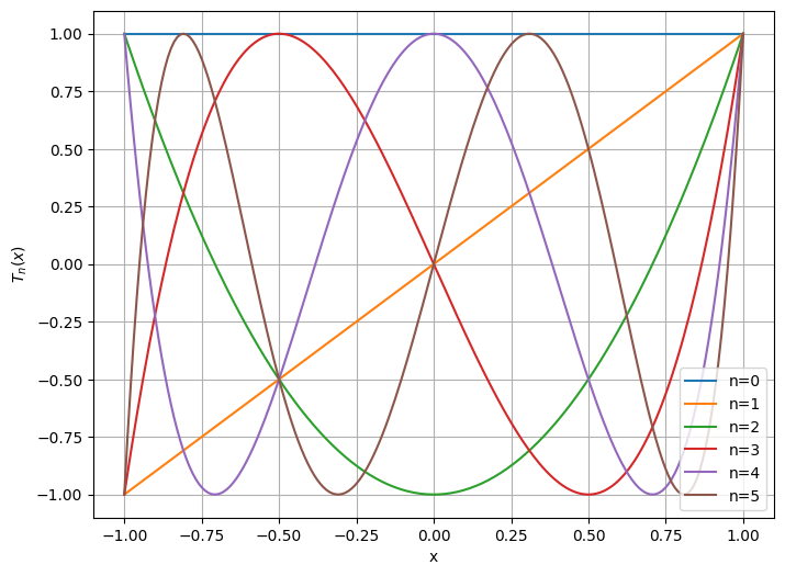
The first few of these are shown below.

Source

N = 200
x = linspace(-1.0,1.0,N)
figure(figsize=(8,6))
for n in range(0,6):
    y = chebyshev(n,x)
    plot(x,y,label='n='+str(n))
legend(), grid(True), xlabel('x'), ylabel('$T_n(x)$');

We can write $x \in [-1,+1]$ in terms of an angle $\theta \in [0,\pi]$

x=\cos\theta

(63)

Properties of Chebyshev polynomials

$T_n(x)$ is a polynomial of degree $n$ .
$T_n(\cos\theta) = \cos(n\theta)$ . (Fourier cosine series)
$T_n(x) = \cos(n\cos^{-1}(x))$
$|T_n(x)| \le 1$
Extrema
$T_n\left(\cos\left(\frac{j\pi}{n}\right)\right) = (-1)^j, \qquad 0 \le j \le n$
(64)
Roots
$T_n\left( \cos \left(\frac{2j+1}{2n}\pi\right) \right) = 0, \qquad 0 \le j \le n-1$
(65)

Proof 5

We prove by contradiction. Suppose that

|p(x)| < 2^{1-n}, \qquad \forall |x| \le 1

(67)

Define

q(x) = 2^{1-n} T_n(x)

(68)

The extrema of $T_n$ are at

x_i = \cos\left( \frac{i\pi}{n} \right), \quad 0 \le i \le n

(69)

and

T_n(x_i) = (-1)^i \qquad \textrm{so that} \qquad q(x_i) = 2^{1-n} (-1)^i

(70)

Now, by assumption

(-1)^i p(x_i) \le |p(x_i)| < 2^{1-n} = (-1)^i q(x_i)

(71)

so that

(-1)^i [q(x_i) - p(x_i)] > 0, \qquad 0 \le i \le n

(72)

$q-p$ changes sign $n$ times, so it must have atleast $n$ distinct roots. But $q-p$ is of degree $n-1$ , and hence we get a contradiction.

6.2.9Optimal nodes¶

Since $\omega_N(x)$ is a monic polynomial of degree $N+1$ , we know from previous theorem that

\max_{-1 \le x \le +1} |\omega_N(x)| \ge 2^{-N}

(73)

Question. Can we choose the $x_i$ so that the minimum value of $2^{-N}$ is achieved ?

Answer. If $\{x_i\}$ are the $N+1$ distinct roots of $T_{N+1}(x)$ , then

\omega_N(x) = 2^{-N} T_{N+1}(x)

(74)

so that

\max_{-1 \le x \le +1} |\omega_N(x)| = 2^{-N} \max_{-1 \le x \le +1} |T_{N+1}(x)| = 2^{-N}

(75)

Thus the optimal nodes are Chebyshev points of first kind

x_i = \cos\left( \frac{2i+1}{2N+2} \pi \right), \qquad 0 \le i \le N

(76)

In terms of θ variable, the spacing between these nodes

\theta_{i+1} - \theta_i = \frac{\pi}{N+1}

(77)

is constant. With these points, we have

-\frac{1}{2^{N}} \le \omega_N(x) \le \frac{1}{2^{N}}, \qquad x \in [-1,1]

(78)

Example 8 (Chebyshev points of first kind)

The roots of degree $n$ Chebyshev polynomial $T_n(x)$ are

x_i = \cos\left( \frac{2i+1}{2n} \pi \right), \qquad i=0,1,\ldots,n-1

(79)

The roots are shown below for $n=10,11,\ldots,19$ .

Source

c = 1
for n in range(10,20):
    j = linspace(0,n-1,n)
    theta = (2*j+1)*pi/(2*n)
    x = cos(theta)
    y = 0*x
    subplot(10,1,c)
    plot(x,y,'.')
    xticks([]); yticks([])
    ylabel(str(n))
    c += 1

Note that the roots are clustered near the end points and are contained in $(-1,1)$ ;

x_0 = \cos\left( \frac{1}{2N+2} \pi \right) < 1, \qquad x_N = \cos\left( \frac{2N+1} {2N+2} \pi \right) > -1

(80)

the endpoints of $[-1,+1]$ are not nodes. The nodes are ordered as $x_0 > x_1 > \ldots > x_N$ . We can reorder them by defining the $x_i$ as in (59).

Remark 4 (Chebyshev points of second kind)

In practice, we dont use the Chebyshev nodes as derived above. The important point is how the points are clustered near the ends of the interval. This type of clustering can be achieved by other node sets. If we want $N+1$ nodes, then divide $[0,\pi]$ into $N$ equal intervals so that

\theta_i = \frac{(N-i)\pi}{N}, \qquad i=0,1,\ldots,N

(82)

and then the nodes are given by

x_i = \cos\theta_i

(83)

These are called Chebyshev points of second kind. In Python they can be obtained as

theta = linspace(0,pi,N+1)
x = -cos(theta)

which returns them in the order

-1 = x_0 < x_1 < \ldots < x_N = +1

(84)

They can also be obtained as projections of uniformly spaced points on the unit circle onto the $x$ -axis.

Source

t = linspace(0,pi,1000)
xx, yy = cos(t), sin(t)
plot(xx,yy)

n = 10
theta = linspace(0,pi,n)
plot(cos(theta),sin(theta),'o')
plot(cos(theta),zeros(n),'sr',label='Chebyshev')
for i in range(n):
    x1 = [cos(theta[i]), cos(theta[i])]
    y1 = [0.0, sin(theta[i])]
    plot(x1,y1,'k--')
plot([-1.1,1.1],[0,0],'-')
legend(), xlabel('x')
axis([-1.1, 1.1, 0.0, 1.1])
axis('equal'), title(str(n)+' Chebyshev points');

Below, we compare the polynomial $\omega_N(x)$ for uniform and Chebyshev points for $N=16$ .

Source

M  = 1000
xx = linspace(-1.0,1.0,M)

N = 16
xu = linspace(-1.0,1.0,N+1)    # uniform points
xc = cos(linspace(0.0,pi,N+1)) # chebyshev points
fu = omega(xu,xx)
fc = omega(xc,xx)
plot(xx,fu,'b-',xx,fc,'r-')
legend(("Uniform","Chebyshev"))
grid(True), title("Degree N = "+str(N));

With Chebyshev points, this function is of similar size throughout the interval.

Exercise 4

Plot the function $\omega_N(x)$ for $N=16$ and for Chebyshev points of first and second kind. Write Python code to produce a plot like this.

N = 16

# First kind
theta1 = pi*(2*arange(0,N+1) + 1)/(2*N + 2)
x1 = cos(theta1)

# Second kind
theta2 = linspace(0,pi,N+1)
x2 = cos(theta2)

x  = linspace(-1,1,1000)
f1 = omega(x1,x)
f2 = omega(x2,x)
figure(figsize=(10,8))
plot(x,f1,label='First kind')
plot(x,f2,label='Second kind')
plot([-1,1],[2**(-N),2**(-N)],'--',label='$y=2^{-N}$')
plot([-1,1],[-2**(-N),-2**(-N)],'--',label='$y=-2^{-N}$')
legend(), grid(True), xlabel('x'), ylabel('$\\omega_N(x)$')
title('Degree N = ' + str(N));

6.2Interpolation using polynomials

6.2.1Interpolation using monomials¶

6.2.1.1Condition number of VVV¶

6.2.2Interpolating polynomials¶

6.2.3Lagrange interpolation¶

6.2.4Error estimate¶

6.2.5Uniformly spaced points¶

6.2.6Difficulty of polynomial interpolation¶

6.2.6.1Size of derivatives¶

6.2.6.2Polynomial factor in error bound¶

6.2.7Distribution of data points¶

6.2.8Chebyshev polynomials¶

6.2.9Optimal nodes¶

6.2.1.1Condition number of $V$ ¶