7.12 Trigonometric interpolation
#%config InlineBackend.figure_format = 'svg'
from pylab import *
A smooth function u : [ 0 , 2 π ] → R u : [0,2\pi] \to \re u : [ 0 , 2 π ] → R
u ( x ) = S u ( x ) = ∑ k = − ∞ ∞ u ^ k ϕ k ( x ) , ϕ k ( x ) = e i k x u(x) = Su(x) = \sum_{k=-\infty}^\infty \hat u_k \phi_k(x), \qquad \phi_k(x) = \ee^{\ii k x} u ( x ) = S u ( x ) = k = − ∞ ∑ ∞ u ^ k ϕ k ( x ) , ϕ k ( x ) = e i k x where
u ^ k = 1 2 π ∫ 0 2 π u ( x ) e − i k x d x \hat u_k = \frac{1}{2\pi} \int_0^{2\pi} u(x) \ee^{-\ii k x} \ud x u ^ k = 2 π 1 ∫ 0 2 π u ( x ) e − i k x d x is the continuous Fourier transform . Recall that { ϕ k } \{ \phi_k \} { ϕ k }
We can truncate the series S u Su S u u ^ k \hat u_k u ^ k u ( x ) u(x) u ( x ) x x x
An approximation method which makes use of the function values at a discrete set of points only, will be more useful in computations.
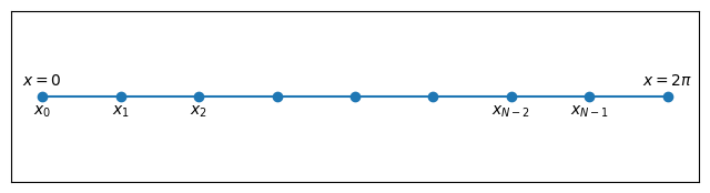
7.12.1 Interpolation problem ¶ For any even integer N > 0 N>0 N > 0 [ 0 , 2 π ] [0,2\pi] [ 0 , 2 π ]
x j = 2 π j N , j = 0 , 1 , … , N − 1 x_j = \frac{2\pi j}{N}, \qquad j=0,1,\ldots,N-1 x j = N 2 πj , j = 0 , 1 , … , N − 1 which are uniformly spaced with spacing
h = 2 π N h = \frac{2\pi}{N} h = N 2 π N = 9
h = 2*pi/N
x = h * arange(0,N)
figure(figsize=(8,2))
plot(x,0*x,'-o')
d = 0.005
text(0,d,"$x=0$",ha='center',va='bottom')
text(x[-1],d,"$x=2\\pi$",ha='center',va='bottom')
text(0,-d,"$x_0$",ha='center',va='top')
text(h,-d,"$x_1$",ha='center',va='top')
text(2*h,-d,"$x_2$",ha='center',va='top')
text(x[-3],-d,"$x_{N-2}$",ha='center',va='top')
text(x[-2],-d,"$x_{N-1}$",ha='center',va='top')
xticks([]), yticks([]);Note that x 0 = 0 x_0 = 0 x 0 = 0 x N − 1 = 2 π − h < 2 π x_{N-1} = 2\pi - h < 2\pi x N − 1 = 2 π − h < 2 π x = 2 π x=2\pi x = 2 π x = 0 x=0 x = 0
In Python, we can generate the grid points like this.
h = 2 * pi / N
x = h * arange(0,N)
The degree N / 2 N/2 N /2
I N u ( x ) = ∑ k = − N / 2 N / 2 − 1 u ~ k ϕ k ( x ) = ∑ k = − N / 2 N / 2 − 1 u ~ k e i k x I_N u(x) = \sumf \tilu_k \phi_k(x) = \sumf \tilu_k \ee^{\ii k x} I N u ( x ) = k = − N /2 ∑ N /2 − 1 u ~ k ϕ k ( x ) = k = − N /2 ∑ N /2 − 1 u ~ k e i k x We will determine the N N N u ~ k \tilu_k u ~ k
u j = u ( x j ) = I N u ( x j ) , j = 0 , 1 , … , N − 1 u_j = u(x_j) = I_N u(x_j), \qquad j=0,1,\ldots,N-1 u j = u ( x j ) = I N u ( x j ) , j = 0 , 1 , … , N − 1 This is a system of N × N N \times N N × N
First prove the orthogonality relation
1 N ∑ j = 0 N − 1 e − i p x j = { 1 , p = N m , m = 0 , ± 1 , ± 2 , … 0 , otherwise \boxed{
\frac{1}{N} \sum_{j=0}^{N-1} \ee^{-\ii p x_j} = \begin{cases}
1, & p = Nm, \quad m=0, \pm 1, \pm 2, \ldots \\
0, & \textrm{otherwise}
\end{cases}
} N 1 j = 0 ∑ N − 1 e − i p x j = { 1 , 0 , p = N m , m = 0 , ± 1 , ± 2 , … otherwise Then computing
∑ j = 0 N − 1 u ( x j ) e − i k x j = ∑ j = 0 N − 1 I N u ( x j ) e − i k x j = ∑ j = 0 N − 1 ∑ l = − N / 2 N / 2 − 1 u ~ l e i l x j e − i k x j = ∑ l = − N / 2 N / 2 − 1 u ~ l ∑ j = 0 N − 1 e i ( l − k ) x j = ∑ l = − N / 2 N / 2 − 1 u ~ l N δ l k \begin{align}
\sum_{j=0}^{N-1} u(x_j) \ee^{-\ii k x_j}
&= \sum_{j=0}^{N-1} \clr{red}{I_N u(x_j)} \ee^{-\ii k x_j} \\
&= \sum_{j=0}^{N-1} \clr{red}{\sum_{l=-N/2}^{N/2-1} \tilde u_l \ee^{\ii l x_j}} \ee^{-\ii k x_j} \\
&= \sum_{l=-N/2}^{N/2-1} \tilde u_l \clr{blue}{\sum_{j=0}^{N-1} \ee^{\ii (l-k)x_j}} \\
&= \sum_{l=-N/2}^{N/2-1} \tilde u_l \clr{blue}{N \delta_{lk}}
\end{align} j = 0 ∑ N − 1 u ( x j ) e − i k x j = j = 0 ∑ N − 1 I N u ( x j ) e − i k x j = j = 0 ∑ N − 1 l = − N /2 ∑ N /2 − 1 u ~ l e i l x j e − i k x j = l = − N /2 ∑ N /2 − 1 u ~ l j = 0 ∑ N − 1 e i ( l − k ) x j = l = − N /2 ∑ N /2 − 1 u ~ l N δ l k we obtain the discrete Fourier coefficients
u ~ k = 1 N ∑ j = 0 N − 1 u j e − i k x j , k = − N / 2 , … , N / 2 − 1 \boxed{\tilu_k = \frac{1}{N} \sum_{j=0}^{N-1} u_j \ee^{-\ii k x_j}, \qquad k=-N/2, \ldots, N/2 - 1} u ~ k = N 1 j = 0 ∑ N − 1 u j e − i k x j , k = − N /2 , … , N /2 − 1 This is known as the discrete Fourier transform (DFT) of { u j } \{ u_j \} { u j }
The interpolation conditions
u j = ∑ k = − N / 2 N / 2 − 1 u ~ k e i k x j , 0 ≤ j ≤ N − 1 \boxed{u_j = \sumf \tilu_k \ee^{\ii k x_j}, \qquad 0 \le j \le N-1} u j = k = − N /2 ∑ N /2 − 1 u ~ k e i k x j , 0 ≤ j ≤ N − 1 will be called the inverse DFT (IDFT) of { u ~ k } \{ \tilu_k \} { u ~ k }
We can derive a Lagrange form of the interpolation as follows.
I N u ( x ) = ∑ k = − N / 2 N / 2 − 1 u ~ k e i k x = 1 N ∑ k = − N / 2 N / 2 − 1 ∑ j = 0 N − 1 u ( x j ) e i k ( x − x j ) = ∑ j = 0 N − 1 u ( x j ) 1 N ∑ k = − N / 2 N / 2 − 1 e i k ( x − x j ) = ∑ j = 0 N − 1 u ( x j ) ψ j ( x ) \begin{aligned}
I_N u(x)
&= \sumf \tilu_k \ee^{\ii k x} \\
&= \frac{1}{N} \sumf \sum_{j=0}^{N-1} u(x_j) \ee^{\ii k (x-x_j)} \\
&= \sum_{j=0}^{N-1} u(x_j) \frac{1}{N} \sumf \ee^{\ii k (x-x_j)} \\
&= \sum_{j=0}^{N-1} u(x_j) \psi_j(x)
\end{aligned} I N u ( x ) = k = − N /2 ∑ N /2 − 1 u ~ k e i k x = N 1 k = − N /2 ∑ N /2 − 1 j = 0 ∑ N − 1 u ( x j ) e i k ( x − x j ) = j = 0 ∑ N − 1 u ( x j ) N 1 k = − N /2 ∑ N /2 − 1 e i k ( x − x j ) = j = 0 ∑ N − 1 u ( x j ) ψ j ( x ) where
ψ j ( x ) = 1 N ∑ k = − N / 2 N / 2 − 1 e i k ( x − x j ) \psi_j(x) = \frac{1}{N} \sumf \ee^{\ii k (x-x_j)} ψ j ( x ) = N 1 k = − N /2 ∑ N /2 − 1 e i k ( x − x j ) The functions ψ j \psi_j ψ j S N S_N S N
ψ j ( x l ) = δ j l , 0 ≤ j , l ≤ N − 1 \psi_j(x_l) = \delta_{jl}, \qquad 0 \le j,l \le N-1 ψ j ( x l ) = δ j l , 0 ≤ j , l ≤ N − 1 Why did we not include the term corresponding to k = N / 2 k=N/2 k = N /2 N N N N N N
ϕ − N / 2 ( x ) = e − i N x / 2 , ϕ N / 2 ( x ) = e i N x / 2 \phi_{-N/2}(x) = \ee^{-\ii Nx/2}, \qquad \phi_{N/2}(x) = \ee^{\ii Nx/2} ϕ − N /2 ( x ) = e − i N x /2 , ϕ N /2 ( x ) = e i N x /2 take the same values at all the nodes x j x_j x j
Let us define the set of trigonometric functions
S N = { v : [ 0 , 2 π ] → R , v = ∑ k = − N / 2 N / 2 − 1 a k ϕ k , a k ∈ C } S_N = \left\{ v : [0,2\pi] \to \re, \quad v = \sumf a_k \phi_k, \quad a_k \in \complex \right\} S N = ⎩ ⎨ ⎧ v : [ 0 , 2 π ] → R , v = k = − N /2 ∑ N /2 − 1 a k ϕ k , a k ∈ C ⎭ ⎬ ⎫ Define the discrete inner product
( u , v ) N = 2 π N ∑ j = 0 N − 1 u ( x j ) v ( x j ) ‾ \ip{u,v}_N = \frac{2\pi}{N} \sum_{j=0}^{N-1} u(x_j) \conj{v(x_j)} ( u , v ) N = N 2 π j = 0 ∑ N − 1 u ( x j ) v ( x j ) and the usual continuous one
( u , v ) = ∫ 0 2 π u ( x ) v ( x ) ‾ d x \ip{u,v} = \int_0^{2\pi} u(x) \conj{v(x)} \ud x ( u , v ) = ∫ 0 2 π u ( x ) v ( x ) d x In fact, the discrete one can be obtained if we apply Trapezoidal rule to the continuous inner product.
Let
u = ∑ k = − N / 2 N / 2 − 1 a k ϕ k , v = ∑ k = − N / 2 N / 2 − 1 b k ϕ k u = \sumf a_k \phi_k, \qquad v = \sumf b_k \phi_k u = k = − N /2 ∑ N /2 − 1 a k ϕ k , v = k = − N /2 ∑ N /2 − 1 b k ϕ k Then
( u , v ) = ∫ 0 2 π u ( x ) v ( x ) ‾ d x = ∑ k ∑ l a k b l ‾ ∫ 0 2 π ϕ k ( x ) ϕ l ( x ) ‾ d x ⏟ 2 π δ k l = 2 π ∑ k = − N / 2 N / 2 − 1 a k b k ‾ \begin{aligned}
\ip{u,v}
&= \int_0^{2\pi} u(x) \conj{v(x)} \ud x \\
&= \sum_k \sum_l a_k \conj{b_l} \underbrace{\int_0^{2\pi} \phi_k(x) \conj{\phi_l(x)}
\ud x}_{2\pi \delta_{kl}} \\
&= 2\pi \sumf a_k \conj{b_k}
\end{aligned} ( u , v ) = ∫ 0 2 π u ( x ) v ( x ) d x = k ∑ l ∑ a k b l 2 π δ k l ∫ 0 2 π ϕ k ( x ) ϕ l ( x ) d x = 2 π k = − N /2 ∑ N /2 − 1 a k b k and
( u , v ) N = 2 π N ∑ j = 0 N − 1 u ( x j ) v ( x j ) ‾ = 2 π N ∑ j = 0 N − 1 u ( x j ) ∑ k = − N / 2 N / 2 − 1 b k ‾ e − i k x j = 2 π ∑ k = − N / 2 N / 2 − 1 ( 1 N ∑ j = 0 N − 1 u ( x j ) e − i k x j ) b k ‾ = 2 π ∑ k = − N / 2 N / 2 − 1 a k b k ‾ \begin{aligned}
\ip{u,v}_N
&= \frac{2\pi}{N} \sum_{j=0}^{N-1} u(x_j) \conj{v(x_j)} \\
&= \frac{2\pi}{N} \sum_{j=0}^{N-1} u(x_j) \sumf \conj{b_k} \ee^{-\ii k x_j} \\
&= 2\pi \sumf \left( \frac{1}{N} \sum_{j=0}^{N-1} u(x_j) \ee^{-\ii k x_j} \right) \conj{b_k} \\
&= 2\pi \sumf a_k \conj{b_k}
\end{aligned} ( u , v ) N = N 2 π j = 0 ∑ N − 1 u ( x j ) v ( x j ) = N 2 π j = 0 ∑ N − 1 u ( x j ) k = − N /2 ∑ N /2 − 1 b k e − i k x j = 2 π k = − N /2 ∑ N /2 − 1 ( N 1 j = 0 ∑ N − 1 u ( x j ) e − i k x j ) b k = 2 π k = − N /2 ∑ N /2 − 1 a k b k As a consequence, ( ⋅ , ⋅ ) N \ip{\cdot,\cdot}_N ( ⋅ , ⋅ ) N S N S_N S N
∥ u ∥ N : = ( u , u ) N = ( u , u ) = ∥ u ∥ , ∀ u ∈ S N \norm{u}_N := \sqrt{\ip{u,u}_N} = \sqrt{\ip{u,u}} = \norm{u}, \qquad \forall u \in S_N ∥ u ∥ N := ( u , u ) N = ( u , u ) = ∥ u ∥ , ∀ u ∈ S N Hence the interpolant satisfies
( I N u − u , v ) N = 0 , ∀ v ∈ S N \ip{I_N u - u, v}_N = 0, \qquad \forall v \in S_N ( I N u − u , v ) N = 0 , ∀ v ∈ S N Thus
I N u I_N u I N u u u u S N S_N S N
The error u − I N u u - I_N u u − I N u S N S_N S N I N u I_N u I N u u u u S N S_N S N ∥ ⋅ ∥ N \norm{\cdot}_N ∥ ⋅ ∥ N
This is also related to the property that { ϕ k ( x ) } \{ \phi_k(x) \} { ϕ k ( x )}
( ϕ j , ϕ k ) N = 2 π δ j k , 0 ≤ j , k ≤ N \ip{\phi_j, \phi_k}_N = 2 \pi \delta_{jk}, \qquad 0 \le j,k \le N ( ϕ j , ϕ k ) N = 2 π δ jk , 0 ≤ j , k ≤ N Define
P N u = ∑ k = − N / 2 N / 2 − 1 u ^ k ϕ k ∈ S N P_N u = \sumf \hatu_k \phi_k \in S_N P N u = k = − N /2 ∑ N /2 − 1 u ^ k ϕ k ∈ S N which is a truncation of the Fourier series S u Su S u
∑ k = − ∞ ∞ = ∑ k = − N / 2 N / 2 − 1 + ∑ ∣ k ∣ ≳ N / 2 \sum_{k=-\infty}^\infty = \sumf + \sumfr k = − ∞ ∑ ∞ = k = − N /2 ∑ N /2 − 1 + ∣ k ∣ ≳ N /2 ∑ The result of Lemma 4
From the smoothness of the function, we have
∣ u ^ k ∣ = O ( 1 ∣ k ∣ m + 1 ) , m ≥ 1 |\hatu_k| = \order{\frac{1}{|k|^{m+1}}}, \qquad m \ge 1 ∣ u ^ k ∣ = O ( ∣ k ∣ m + 1 1 ) , m ≥ 1 The first inequality is easy since
u − P N u = ∑ ∣ k ∣ ≳ N / 2 u ^ k ϕ k ⟹ ∥ u − P N u ∥ ∞ ≤ ∑ ∣ k ∣ ≳ N / 2 ∣ u ^ k ∣ u - P_N u = \sumfr \hatu_k \phi_k \quad\Longrightarrow\quad \norm{u - P_N u}_\infty \le \sumfr |\hatu_k| u − P N u = ∣ k ∣ ≳ N /2 ∑ u ^ k ϕ k ⟹ ∥ u − P N u ∥ ∞ ≤ ∣ k ∣ ≳ N /2 ∑ ∣ u ^ k ∣ For the second, we use the decomposition
u − I N u = u − P N u − R N u u - I_N u = u - P_N u - R_N u u − I N u = u − P N u − R N u so that
∥ u − I N u ∥ ∞ ≤ ∥ u − P N u ∥ ∞ + ∥ R N u ∥ ∞ \norm{u - I_N u}_\infty \le \norm{u - P_N u}_\infty + \norm{R_N u}_\infty ∥ u − I N u ∥ ∞ ≤ ∥ u − P N u ∥ ∞ + ∥ R N u ∥ ∞ But
∥ R N u ∥ ∞ ≤ ∑ k = − N / 2 N / 2 − 1 ∑ m = − ∞ , m ≠ 0 ∞ ∣ u ^ k + N m ∣ = ∑ ∣ k ∣ ≳ N / 2 ∣ u ^ k ∣ \norm{R_N u}_\infty \le \sumf \sum_{m=-\infty,m\ne 0}^\infty |\hatu_{k+Nm}| =
\sumfr |\hatu_k| ∥ R N u ∥ ∞ ≤ k = − N /2 ∑ N /2 − 1 m = − ∞ , m = 0 ∑ ∞ ∣ u ^ k + N m ∣ = ∣ k ∣ ≳ N /2 ∑ ∣ u ^ k ∣ and hence
∥ u − I N u ∥ ∞ ≤ ∑ ∣ k ∣ ≳ N / 2 ∣ u ^ k ∣ + ∑ ∣ k ∣ ≳ N / 2 ∣ u ^ k ∣ = 2 ∑ ∣ k ∣ ≳ N / 2 ∣ u ^ k ∣ \norm{u - I_N u}_\infty \le \sumfr |\hatu_k| + \sumfr |\hatu_k| = 2 \sumfr |\hatu_k| ∥ u − I N u ∥ ∞ ≤ ∣ k ∣ ≳ N /2 ∑ ∣ u ^ k ∣ + ∣ k ∣ ≳ N /2 ∑ ∣ u ^ k ∣ = 2 ∣ k ∣ ≳ N /2 ∑ ∣ u ^ k ∣ The error is given by
∑ ∣ k ∣ ≳ N / 2 ∣ u ^ k ∣ ≤ C [ 1 ( N / 2 ) m + 1 + 1 ( N / 2 + 1 ) m + 1 + … ] \sumfr |\hatu_k| \le C \left[ \frac{1}{(N/2)^{m+1}} + \frac{1}{(N/2+1)^{m+1}} + \ldots \right] ∣ k ∣ ≳ N /2 ∑ ∣ u ^ k ∣ ≤ C [ ( N /2 ) m + 1 1 + ( N /2 + 1 ) m + 1 1 + … ] The sum on the right can be bounded by an integral
1 ( N / 2 ) m + 1 + 1 ( N / 2 + 1 ) m + 1 + … < ∫ 0 ∞ 1 ( N / 2 + x − 1 ) m + 1 d x = 1 m ( N / 2 − 1 ) m = O ( 1 N m ) for N ≫ 1 \begin{aligned}
\frac{1}{(N/2)^{m+1}} + \frac{1}{(N/2+1)^{m+1}} + \ldots
&< \int_0^\infty \frac{1}{(N/2 + x - 1)^{m+1}} \ud x \\
&= \frac{1}{m(N/2-1)^{m}} \\
&= \order{\frac{1}{N^{m}}} \quad \textrm{for } N \gg 1
\end{aligned} ( N /2 ) m + 1 1 + ( N /2 + 1 ) m + 1 1 + … < ∫ 0 ∞ ( N /2 + x − 1 ) m + 1 1 d x = m ( N /2 − 1 ) m 1 = O ( N m 1 ) for N ≫ 1 7.12.2 Computing the DFT ¶ 7.12.2.1 DFT of a real function ¶ If the function u u u
u ~ − k = u ~ k ‾ , 1 ≤ k ≤ N / 2 − 1 \tilu_{-k} = \conj{\tilu_k}, \qquad 1 \le k \le N/2-1 u ~ − k = u ~ k , 1 ≤ k ≤ N /2 − 1 and u ~ 0 \tilu_0 u ~ 0 u ~ − N / 2 \tilu_{-N/2} u ~ − N /2
u ~ 0 = 1 N ∑ j = 0 N − 1 u ( x j ) \tilu_0 = \frac{1}{N} \sum_{j=0}^{N-1} u(x_j) u ~ 0 = N 1 j = 0 ∑ N − 1 u ( x j ) which is real, and
u ~ − N / 2 = 1 N ∑ j = 0 N − 1 u ( x j ) e i π j = 1 N ∑ j = 0 N − 1 u ( x j ) cos ( π j ) \tilu_{-N/2} = \frac{1}{N} \sum_{j=0}^{N-1} u(x_j) \ee^{\ii \pi j} = \frac{1}{N} \sum_{j=0}^{N-1} u(x_j) \cos(\pi j) u ~ − N /2 = N 1 j = 0 ∑ N − 1 u ( x j ) e i πj = N 1 j = 0 ∑ N − 1 u ( x j ) cos ( πj ) is also real. When we want to evaluate I N u ( x ) I_N u(x) I N u ( x ) x x x
I N u ( x ) = u ~ 0 + ∑ k = 1 N / 2 − 1 ( u ~ k ϕ k ( x ) + u ~ k ϕ k ( x ) ‾ ) + u ~ − N / 2 ϕ − N / 2 ( x ) I_N u(x) = \tilu_0 + \sum_{k=1}^{N/2-1} \left( \tilu_k \phi_k(x) + \conj{\tilu_k \phi_k(x)} \right) + \tilu_{-N/2} \phi_{-N/2}(x) I N u ( x ) = u ~ 0 + k = 1 ∑ N /2 − 1 ( u ~ k ϕ k ( x ) + u ~ k ϕ k ( x ) ) + u ~ − N /2 ϕ − N /2 ( x ) the above expression is not real because of the last term. We can modify it as
I N u ( x ) = u ~ 0 + ∑ k = 1 N / 2 − 1 ( u ~ k ϕ k ( x ) + u ~ k ϕ k ( x ) ‾ ) + 1 2 u ~ − N / 2 ϕ − N / 2 ( x ) + 1 2 u ~ − N / 2 ϕ N / 2 ( x ) \begin{align}
I_N u(x) &= \tilu_0 + \sum_{k=1}^{N/2-1} \left( \tilu_k \phi_k(x) + \conj{\tilu_k \phi_k(x)} \right) \\
& \qquad + \half \tilu_{-N/2} \phi_{-N/2}(x) + \half \tilu_{-N/2} \phi_{N/2}(x)
\end{align} I N u ( x ) = u ~ 0 + k = 1 ∑ N /2 − 1 ( u ~ k ϕ k ( x ) + u ~ k ϕ k ( x ) ) + 2 1 u ~ − N /2 ϕ − N /2 ( x ) + 2 1 u ~ − N /2 ϕ N /2 ( x ) i.e.,
I N u ( x ) = ∑ k = − N / 2 N / 2 ′ u ^ k ϕ k ( x ) , u ^ N / 2 = u ^ − N / 2 I_N u(x) = {\sum_{k=-N/2}^{N/2}}^\prime \hatu_k \phi_k(x), \qquad \hatu_{N/2} = \hatu_{-N/2} I N u ( x ) = k = − N /2 ∑ N /2 ′ u ^ k ϕ k ( x ) , u ^ N /2 = u ^ − N /2 and the prime denotes that the first and last terms must be multiplied by half. This ensures that the interpolation conditions are still satisfied and I N u ( x ) I_N u(x) I N u ( x ) x ∈ [ 0 , 2 π ] x \in [0,2\pi] x ∈ [ 0 , 2 π ]
However, in actual numerical computation, we may get an imaginary part of order machine precision, and then we have to take the real part. Then, we may as well compute it as before and take real part
I N u ( x ) = Real ∑ k = − N / 2 N / 2 − 1 u ~ k ϕ k ( x ) I_N u (x) = \textrm{Real} \sumf \tilu_k \phi_k(x) I N u ( x ) = Real k = − N /2 ∑ N /2 − 1 u ~ k ϕ k ( x ) Computing each u ~ k \tilu_k u ~ k (9) O ( N ) \order{N} O ( N ) N N N O ( N 2 ) \order{N^2} O ( N 2 ) N × N N \times N N × N
[ u ( x 0 ) , u ( x 1 ) , … , u ( x N − 1 ) ] ⊤ [u(x_0), \ u(x_1), \ \ldots, \ u(x_{N-1})]^\top [ u ( x 0 ) , u ( x 1 ) , … , u ( x N − 1 ) ] ⊤ The matrix has special structure and using some tricks, the cost can be reduced to O ( N log N ) \order{N \log N} O ( N log N ) Cooley & Tukey, 1965
7.12.2.3 FFT using Numpy ¶ Numpy has routines to compute the DFT using FFT, see numpy.fft . It takes the trigonometric polynomial in the form
I N u ( x ) = 1 N ∑ k = − N / 2 + 1 N / 2 u ~ k e i k x , x ∈ [ 0 , 2 π ] I_N u(x) = \frac{1}{N} \sum_{k=-N/2+1}^{N/2} \tilu_k \ee^{\ii k x}, \qquad x \in [0,2\pi] I N u ( x ) = N 1 k = − N /2 + 1 ∑ N /2 u ~ k e i k x , x ∈ [ 0 , 2 π ] which is different from our convention.
from numpy import pi,arange
import numpy.fft as fft
h = 2*pi/N
x = h*arange(0,N)
u = f(x)
u_hat = fft(u)
The output u_hat gives the DFT in the following order
u ~ k = u ~ 0 , u ~ 1 , … , u ~ N / 2 , u ~ − N / 2 + 1 , … , u ~ − 2 , u ~ − 1 \tilu_k = \tilu_0, \ \tilu_1, \ \ldots, \ \tilu_{N/2}, \ \tilu_{-N/2+1}, \ \ldots, \ \tilu_{-2}, \ \tilu_{-1} u ~ k = u ~ 0 , u ~ 1 , … , u ~ N /2 , u ~ − N /2 + 1 , … , u ~ − 2 , u ~ − 1 Scipy.fft also provides equivalent routines for FFT.
See more examples of using Fourier interpolation for approximation and differentiation here http:// .
7.12.3 Examples ¶ The following function computes the trigonometric interpolant and plots it. It also computes error norm by using ne uniformly spaced points.
# Wave numbers are arranged as k=[0,1,...,N/2,-N/2+1,-N/2,...,-1]
def fourier_interp(N,f,ne=1000,fig=True):
    if mod(N,2) != 0:
        print("N must be even")
        return
    h = 2*pi/N; x = h*arange(0,N);
    v = f(x);
    v_hat = fft(v)
    k = zeros(N)
    n = N//2
    k[0:n+1] = arange(0,n+1)
    k[n+1:] = arange(-n+1,0,1)

    xx = linspace(0.0,2*pi,ne)
    vf = real(exp(1j*outer(xx,k)) @ v_hat) / N
    ve = f(xx)

    # Plot interpolant and exact function
    if fig:
        plot(x,v,'o',xx,vf,xx,ve)
        legend(('Data','Fourier','Exact'))
        xlabel('x'), ylabel('y'), title("N = "+str(N))

    errori = abs(vf-ve).max()
    error2 = sqrt(h*sum((vf-ve)**2))
    print("Error (max,L2) = ",errori,error2)
    return errori, error2
To measure rate of error convergence, we can compute error with N N N 2 N 2N 2 N
E N = C N m , E 2 N = C ( 2 N ) m E_N = \frac{C}{N^m}, \qquad E_{2N} = \frac{C}{(2N)^m} E N = N m C , E 2 N = ( 2 N ) m C and estimate the rate
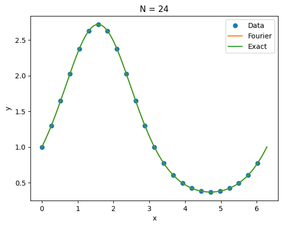
m = log ( E N / E 2 N ) log 2 m = \frac{\log(E_N / E_{2N})}{\log 2} m = log 2 log ( E N / E 2 N ) 7.12.3.1 Infinitely smooth, periodic function ( m = ∞ ) (m = \infty) ( m = ∞ ) ¶ u ( x ) = exp ( sin x ) , x ∈ [ 0 , 2 π ] u(x) = \exp(\sin x), \qquad x \in [0,2\pi] u ( x ) = exp ( sin x ) , x ∈ [ 0 , 2 π ] f1 = lambda x: exp(sin(x))
fourier_interp(24,f1);Error (max,L2) = 7.993605777301127e-14 6.463175355583166e-13
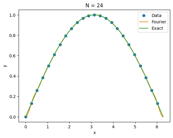
7.12.3.2 Infinitely smooth, derivative not periodic ( m = 1 ) (m = 1) ( m = 1 ) ¶ u ( x ) = sin ( x / 2 ) , x ∈ [ 0 , 2 π ] u(x) = \sin(x/2), \qquad x \in [0,2\pi] u ( x ) = sin ( x /2 ) , x ∈ [ 0 , 2 π ] g = lambda x: sin(x/2)
e1i,e12 = fourier_interp(24,g)Error (max,L2) = 0.024834020843920963 0.09773746633443824
e2i,e22 = fourier_interp(48,g,fig=False)
print("Rate  (max,L2) = ", log(e1i/e2i)/log(2), log(e12/e22)/log(2))
Error (max,L2) = 0.012408518426188423 0.024996075910098184
Rate (max,L2) = 1.0009869969530465 1.9672100793199772
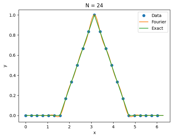
7.12.3.3 Continuous function ( m = 1 ) (m = 1) ( m = 1 ) ¶ f ( x ) = { 1 − 2 π ∣ x − π ∣ , π / 2 ≤ x ≤ 3 π / 2 0 , otherwise , x ∈ [ 0 , 2 π ] f(x) = \begin{cases}
1 - \frac{2}{\pi} |x - \pi|, & \pi/2 \le x \le 3\pi/2 \\
0, & \textrm{otherwise}
\end{cases}, \qquad x \in [0,2\pi] f ( x ) = { 1 − π 2 ∣ x − π ∣ , 0 , π /2 ≤ x ≤ 3 π /2 otherwise , x ∈ [ 0 , 2 π ] trihat = lambda x: (x >= 0.5*pi)*(x <= 1.5*pi)*(1 - 2*abs(x-pi)/pi)
e1i,e12 = fourier_interp(24,trihat)Error (max,L2) = 0.03193459816557198 0.15767834270061085
e2i,e22 = fourier_interp(48,trihat,fig=False)
print("Rate  (max,L2) = ", log(e1i/e2i)/log(2), log(e12/e22)/log(2))
Error (max,L2) = 0.01586894831194785 0.03976512461360404
Rate (max,L2) = 1.0089137779952295 1.987408920855071
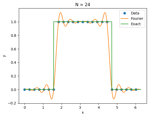
7.12.3.4 Discontinuous function ( m = 0 ) (m=0) ( m = 0 ) ¶ Lemma 6
f ( x ) = { 1 , π / 2 < x < 3 π / 2 0 , otherwise , x ∈ [ 0 , 2 π ] f(x) = \begin{cases}
1, & \pi/2 < x < 3\pi/2 \\
0, & \textrm{otherwise}
\end{cases}, \qquad x \in [0,2\pi] f ( x ) = { 1 , 0 , π /2 < x < 3 π /2 otherwise , x ∈ [ 0 , 2 π ] f2 = lambda x: (abs(x-pi) < 0.5*pi)
e1i,e12 = fourier_interp(24,f2)Error (max,L2) = 0.9957898426758144 2.8589545556697407
e2i,e22 = fourier_interp(48,f2)
print("Rate  (max,L2) = ", log(e1i/e2i)/log(2), log(e12/e22)/log(2))
Error (max,L2) = 0.9915466799725409 1.4514563367440128
Rate (max,L2) = 0.006160606441865679 0.9779865149620691
We do not get convergence in maximum norm but we see convergence in 2-norm at a rate of 1 / N 1/N 1/ N
Uniformly spaced points were not a good choice for polynomial interpolation, since they lead to Runge phenomenon. We needed to use points clustered at the boundaries to get good approximations.
Uniformly spaced points are the best choice for trigonometric interpolation. They lead to discrete orthogonality and an explicit expression for the DFT. Moreover, the highly efficient FFT is also possible because of this property.
With N = 100 , 500 N=100,500 N = 100 , 500 ∣ u ~ k ∣ |\tilu_k| ∣ u ~ k ∣ k k k 0 ≤ k ≤ N / 2 0 \le k \le N/2 0 ≤ k ≤ N /2
u ( x ) = sin ( 10 x ) + sin ( 50 x ) , x ∈ [ 0 , 2 π ] u(x) = \sin(10x) + \sin(50x), \qquad x \in [0,2\pi] u ( x ) = sin ( 10 x ) + sin ( 50 x ) , x ∈ [ 0 , 2 π ] Comment on the nature of these curves.
To test convergence as N → ∞ N \to \infty N → ∞ I N u I_N u I N u { x j } \{ x_j \} { x j } m = 1000 m = 1000 m = 1000
∥ I N u − u ∥ ∞ ≈ max j ∣ I N u ( x j ) − u ( x j ) ∣ ∥ I N u − u ∥ 2 ≈ ( 2 π m ∑ j [ I N u ( x j ) − u ( x j ) ] 2 ) 1 2 \begin{align}
\norm{I_N u - u}_\infty &\approx \max_{j} |I_N u(x_j) - u(x_j)| \\
\norm{I_N u - u}_2 &\approx \left( \frac{2\pi}{m} \sum_{j} [I_N u(x_j) - u(x_j)]^2 \right)^\half
\end{align} ∥ I N u − u ∥ ∞ ∥ I N u − u ∥ 2 ≈ j max ∣ I N u ( x j ) − u ( x j ) ∣ ≈ ( m 2 π j ∑ [ I N u ( x j ) − u ( x j ) ] 2 ) 2 1 Plot error versus N N N
If u ^ k \hatu_k u ^ k u ( x ) u(x) u ( x ) u ′ ( x ) u'(x) u ′ ( x ) i k u ^ k \ii k \hatu_k i k u ^ k u ~ k \tilu_k u ~ k i k u ~ k \ii k \tilu_k i k u ~ k u ′ ( x ) u'(x) u ′ ( x )
{ u j } ⟶ D F T { u ~ k } ⟶ { i k u ~ k } ⟶ I D F T { u j ′ } \{ u_j \} \overset{DFT}{\longrightarrow} \{ \tilu_k \} \longrightarrow \{ \ii k \tilu_k \} \overset{IDFT}{\longrightarrow} \{ u_j' \} { u j } ⟶ D FT { u ~ k } ⟶ { i k u ~ k } ⟶ I D FT { u j ′ } We can thus compute derivatives at all points with almost O ( N ) \order{N} O ( N )
Cooley, J. W., & Tukey, J. W. (1965). An algorithm for the machine calculation of complex Fourier series. Mathematics of Computation , 19 (90), 297–301. 10.1090/S0025-5718-1965-0178586-1 Brunton, S. L., & Kutz, J. N. (2019). Data-Driven Science and Engineering: Machine Learning, Dynamical Systems, and Control (1st ed.). Cambridge University Press. 10.1017/9781108380690