7.6 Chebyshev approximation
from pylab import *
from scipy.interpolate import barycentric_interpolate
Trefethen, 2019
7.6.1 Chebyshev series ¶ If f : [ − 1 , 1 ] → R f : [-1,1] \to \re f : [ − 1 , 1 ] → R
f ( x ) = ∑ k = 0 ∞ a k T k ( x ) f(x) = \sum_{k=0}^\infty a_k T_k(x) f ( x ) = k = 0 ∑ ∞ a k T k ( x ) which is absolutely and uniformly convergent. The coefficients are given by
a 0 = 1 π ∫ − 1 1 f ( x ) 1 − x 2 d x , a k = 2 π ∫ − 1 1 f ( x ) T k ( x ) 1 − x 2 d x , k ≥ 1 a_0 = \frac{1}{\pi} \int_{-1}^1 \frac{f(x)}{\sqrt{1-x^2}} \ud x, \qquad
a_k = \frac{2}{\pi} \int_{-1}^1 \frac{f(x) T_k(x)}{\sqrt{1-x^2}} \ud x, \qquad k \ge 1 a 0 = π 1 ∫ − 1 1 1 − x 2 f ( x ) d x , a k = π 2 ∫ − 1 1 1 − x 2 f ( x ) T k ( x ) d x , k ≥ 1 For any integer ν ≥ 0 \nu \ge 0 ν ≥ 0 f f f f ( ν − 1 ) f^{(\nu-1)} f ( ν − 1 ) [ − 1 , 1 ] [-1,1] [ − 1 , 1 ] ν \nu ν f ( ν ) f^{(\nu)} f ( ν ) V V V k ≥ ν + 1 k \ge \nu + 1 k ≥ ν + 1 f f f
∣ a k ∣ ≤ 2 V π k ( k − 1 ) … ( k − ν ) ≤ 2 V π ( k − ν ) ν + 1 |a_k| \le \frac{2 V}{\pi k (k-1) \ldots (k-\nu)} \le \frac{2V}{\pi(k - \nu)^{\nu+1}} ∣ a k ∣ ≤ πk ( k − 1 ) … ( k − ν ) 2 V ≤ π ( k − ν ) ν + 1 2 V 7.6.2 Projection and interpolation ¶ The Chebyshev projection is obtained by truncating the Chebyshev series
f n ( x ) = ∑ k = 0 n a k T k ( x ) f_n(x) = \sum_{k=0}^n a_k T_k(x) f n ( x ) = k = 0 ∑ n a k T k ( x ) Let p n ( x ) p_n(x) p n ( x ) f ( x ) f(x) f ( x ) n + 1 n+1 n + 1 { x j } \{ x_j \} { x j }
p n ( x ) = ∑ k = 0 n c k T k ( x ) p_n(x) = \sum_{k=0}^n c_k T_k(x) p n ( x ) = k = 0 ∑ n c k T k ( x ) The coefficients c k c_k c k p n ( x j ) = f ( x j ) p_n(x_j) = f(x_j) p n ( x j ) = f ( x j ) j = 0 , 1 , … , n j=0,1,\ldots,n j = 0 , 1 , … , n
7.6.2.1 Differentiable functions ¶ If f f f Theorem 2 V V V f ( ν ) f^{(\nu)} f ( ν ) ν ≥ 1 \nu \ge 1 ν ≥ 1 n > ν n > \nu n > ν
∥ f − f n ∥ ∞ ≤ 2 V π ν ( n − ν ) ν \norm{f - f_n}_\infty \le \frac{2 V}{\pi \nu (n - \nu)^\nu} ∥ f − f n ∥ ∞ ≤ π ν ( n − ν ) ν 2 V and its Chebyshev interpolants satisfy
∥ f − p n ∥ ∞ ≤ 4 V π ν ( n − ν ) ν \norm{f - p_n}_\infty \le \frac{4 V}{\pi \nu (n - \nu)^\nu} ∥ f − p n ∥ ∞ ≤ π ν ( n − ν ) ν 4 V Thus f ( ν ) f^{(\nu)} f ( ν ) O ( n − ν ) \order{n^{-\nu}} O ( n − ν ) n → ∞ n \to \infty n → ∞
For ν = 0 \nu = 0 ν = 0 f ( x ) = sign ( x ) f(x) = \textrm{sign}(x) f ( x ) = sign ( x )
Even the projections do not converge, since
∣ a k ∣ = O ( 1 k ) , f ( x ) − f n ( x ) = ? ∑ k = n + 1 ∞ a k T k ( x ) |a_k| = \order{ \frac{1}{k} }, \qquad f(x) - f_n(x) \overset{?}{=} \sum_{k=n+1}^\infty a_k T_k(x) ∣ a k ∣ = O ( k 1 ) , f ( x ) − f n ( x ) = ? k = n + 1 ∑ ∞ a k T k ( x ) and
∥ f − f n ∥ ∞ ≤ ∑ k = n + 1 ∞ ∣ a k ∣ ↛ 0 \norm{f - f_n}_\infty \le \sum_{k=n+1}^\infty |a_k| \not\to 0 ∥ f − f n ∥ ∞ ≤ k = n + 1 ∑ ∞ ∣ a k ∣ → 0 since ∑ k ( 1 / k ) \sum_k (1/k) ∑ k ( 1/ k )
f = lambda x: sign(x)
xp = linspace(-1,1,1000)
for n in [11,21,41]:
    theta = linspace(0,pi,n+1)
    x = -cos(theta)
    y = f(x)
    yp = barycentric_interpolate(x,y,xp)
    plot(xp,yp,label='n='+str(n))
plot(xp,f(xp),label='Exact')
legend(), xlabel('x'), ylabel('y');
On the average, the error decreases, but around x = 0 x=0 x = 0
For ν = 1 \nu = 1 ν = 1 f ( x ) = ∣ x ∣ f(x) = |x| f ( x ) = ∣ x ∣ V = 2 V=2 V = 2
∥ f − f n ∥ ∞ ≤ 4 π ( n − 1 ) , ∥ f − p n ∥ ∞ ≤ 8 π ( n − 1 ) \norm{f - f_n}_\infty \le \frac{4}{\pi(n-1)}, \qquad \norm{f - p_n}_\infty \le \frac{8}{\pi (n-1)} ∥ f − f n ∥ ∞ ≤ π ( n − 1 ) 4 , ∥ f − p n ∥ ∞ ≤ π ( n − 1 ) 8 The degree 10 interpolant looks like this.
f = lambda x: abs(x)
n = 10
xp = linspace(-1,1,1000)
theta = linspace(0,pi,n+1)
x = -cos(theta)
y = f(x)
yp = barycentric_interpolate(x,y,xp)
plot(x,y,'o',label='Data')
plot(xp,f(xp),label='Exact')
plot(xp,yp,label='Interpolant')
legend(), xlabel('x'), ylabel('y')
title('Degree '+str(n)+' interpolant');
Now compute error norm for increasing degree. The norm is only an approximation.
n = 10
nvalues,evalues = [],[]
for i in range(10):
    theta = linspace(0,pi,n+1)
    x = -cos(theta)
    y = f(x)
    yp = barycentric_interpolate(x,y,xp)
    e = abs(f(xp) - yp).max()
    nvalues.append(n), evalues.append(e)
    n = 2 * n
nvalues = array(nvalues)
loglog(nvalues,evalues,'o-',label="Error")
loglog(nvalues, 8/(pi*(nvalues-1)),label="$8/(\\pi (n-1))$")
legend(), xlabel('n'), ylabel('$||f-p_n||$');
In log-log scale, we see that log ∥ f − p n ∥ ∞ \log\norm{f-p_n}_\infty log ∥ f − p n ∥ ∞ log ( n ) \log(n) log ( n )
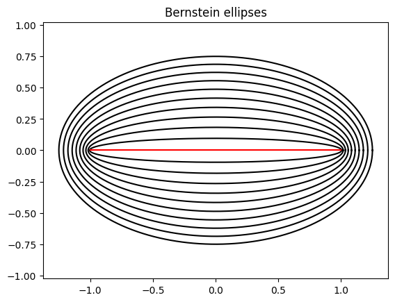
7.6.2.2 Analytic functions ¶ For any ρ > 1 \rho > 1 ρ > 1 E ρ E_\rho E ρ x = − 1 x=-1 x = − 1 x = + 1 x=+1 x = + 1
ρ = semi-minor axis + semi-major axis \rho = \textrm{semi-minor axis + semi-major axis} ρ = semi-minor axis + semi-major axis It can be obtained by mapping the circle of radius ρ \rho ρ ξ = ρ exp ( i θ ) \xi = \rho \exp(\ii \theta) ξ = ρ exp ( i θ )
z = 1 2 ( ξ + ξ − 1 ) z = \half (\xi + \xi^{-1}) z = 2 1 ( ξ + ξ − 1 ) theta = linspace(0,2*pi,500)
for rho in arange(1.1,2.1,0.1):
xi = rho * exp(1j * theta)
z = 0.5 * (xi + 1/xi)
plot(real(z), imag(z),'k-')
plot([-1,1],[0,0],'r-'), axis('equal')
title('Bernstein ellipses');Let f : [ − 1 , 1 ] → R f : [-1,1] \to \re f : [ − 1 , 1 ] → R E ρ E_\rho E ρ ρ > 1 \rho > 1 ρ > 1 ∣ f ( x ) ∣ ≤ M |f(x)| \le M ∣ f ( x ) ∣ ≤ M M M M
∣ a 0 ∣ ≤ M , ∣ a k ∣ ≤ 2 M ρ k , k ≥ 1 |a_0| \le M, \qquad |a_k| \le \frac{2M}{\rho^k}, \qquad k \ge 1 ∣ a 0 ∣ ≤ M , ∣ a k ∣ ≤ ρ k 2 M , k ≥ 1 If f f f Theorem 4 n ≥ 0 n \ge 0 n ≥ 0
∥ f − f n ∥ ∞ ≤ 2 M ρ − n ρ − 1 \norm{f - f_n}_\infty \le \frac{2 M \rho^{-n}}{\rho - 1} ∥ f − f n ∥ ∞ ≤ ρ − 1 2 M ρ − n and its Chebyshev interpolants satisfy
∥ f − p n ∥ ∞ ≤ 4 M ρ − n ρ − 1 \norm{f - p_n}_\infty \le \frac{4 M \rho^{-n}}{\rho - 1} ∥ f − p n ∥ ∞ ≤ ρ − 1 4 M ρ − n We interpolate the function f ( x ) = 1 / ( 1 + 16 x 2 ) f(x) = 1/(1+16 x^2) f ( x ) = 1/ ( 1 + 16 x 2 ) [ − 1 , 1 ] [-1,1] [ − 1 , 1 ]
f = lambda x: 1.0/(1.0 + 16 * x**2)
n = 10
nvalues,evalues = [],[]
for i in range(10):
    theta = linspace(0,pi,n+1)
    x = -cos(theta)
    y = f(x)
    yp = barycentric_interpolate(x,y,xp)
    e = abs(f(xp) - yp).max()
    nvalues.append(n), evalues.append(e)
    n = n + 10
nvalues = array(nvalues)
semilogy(nvalues,evalues,'o-',label="Error")
legend(), xlabel('n'), ylabel('$||f-p_n||$');
We see that log ∥ f − p n ∥ ∞ \log\norm{f - p_n}_\infty log ∥ f − p n ∥ ∞ n n n n n n
Trefethen, L. N. (2019). Approximation Theory and Approximation Practice, Extended Edition . Society for Industrial. 10.1137/1.9781611975949