Piecewise polynomial interpolation

#%config InlineBackend.figure_format = 'svg'
from pylab import *
from matplotlib import animation
from IPython.display import HTML

Consider a partition of $[a,b]$ into a grid

a = x_0 < x_1 < \ldots < x_N = b

(1)

The points $x_j$ are called knots, breakpoints or nodes. Let $p(x)$ be a polynomial on each of the subintervals/elements/cells

[x_0,x_1], \quad [x_1,x_2], \quad \ldots, [x_{N-1},x_N]

(2)

i.e.,

p(x) \in \poly_r, \qquad x \in [x_i,x_{i+1}]

(3)

Note that $p(x)$ need not be a polynomial in $[a, b]$ .

In general, no restrictions on the continuity of $p(x)$ or its derivatives at the end points of the sub-intervals might exist. Putting additional continuity constraints leads to different types of approximations. In this chapter, we are interested in globally continuous approximations.

6.9.1Piecewise linear interpolation¶

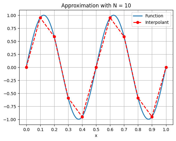
Let us demand the we want a continuous approximation. We are given the function values $y_i = f(x_i)$ at all the nodes of our grid. We can construct the polynomial in each sub-interval

p(x) = \frac{x - x_{i+1}}{x_i - x_{i+1}} y_i + \frac{x - x_i}{x_{i+1} - x_i} y_{i+1}, \qquad x_i \le x \le x_{i+1}

(4)

Clearly, such a function is piecewise linear and continuous in the whole domain. Here is the approximation with $N=10$ intervals of $f(x) = \sin(4 \pi x)$ for $x \in [0,1]$ .

fun = lambda x: sin(4*pi*x)
xmin, xmax = 0.0, 1.0
N = 10
x = linspace(xmin,xmax,N+1)
f = fun(x)

xe = linspace(xmin,xmax,100) # for plotting only
fe = fun(xe)

fig, ax = subplots()
line1, = ax.plot(xe,fe,'-',linewidth=2,label='Function')
line2, = ax.plot(x,f,'or--',linewidth=2,label='Interpolant')
ax.set_xticks(x), ax.grid()
ax.set_xlabel('x'), ax.legend()
ax.set_title('Approximation with N = ' + str(N));

The vertical grid lines show the boundaries of the sub-intervals.

From the error estimate of polynomial interpolation,

f(x) - p(x) = \frac{1}{2!} (x-x_i)(x - x_{i+1}) f''(\xi), \qquad \xi \in [x_i, x_{i+1}]

(5)

we get the local interpolation error estimate

\max_{x \in [x_i,x_{i+1}]} |f(x) - p(x)| \le \frac{h_{i+1}^2}{8} \max_{t \in [x_i,x_{i+1}]} |f''(t)|, \qquad h_{i+1} = x_{i+1} - x_i

(6)

from which we get the global error

\max_{x \in [a,b]} |f(x) - p(x)| \le \frac{h^2}{8} \max_{t \in [a,b]} |f''(t)|, \qquad h = \max_i h_i

(7)

Clearly, we have convergence as $N \to \infty$ , $h \to 0$ . The convergence is quadratic; if $h$ becomes $h/2$ , the error reduces by a factor of $1/4$ .

6.9.1.1Finite element form¶

We have written down the polynomial in a piecewise manner but we can also write a global view of the polynomial by defining some basis functions. Since

x \in [x_i, x_{i+1}]: \qquad p(x) = \clr{red}{\frac{x - x_{i+1}}{x_i - x_{i+1}}} y_i + \frac{x - x_i}{x_{i+1} - x_i} y_{i+1}

(8)

and similarly

x \in [x_{i-1}, x_{i}]: \qquad p(x) = \frac{x - x_{i}}{x_{i-1} - x_{i}} y_{i-1} + \clr{red}{\frac{x - x_{i-1}}{x_{i} - x_{i-1}}} y_{i}

(9)

Let us define

\phi_i(x) = \begin{cases} \frac{x - x_{i-1}}{x_i - x_{i-1}}, & x_{i-1} \le x \le x_i \\ \frac{x_{i+1} - x}{x_{i+1} - x_i}, & x_i \le x \le x_{i+1} \\ 0, & \textrm{otherwise} \end{cases}

(10)

These are triangular hat functions with compact support. Then the piecewise linear approximation is given by

p(x) = \sum_{i=0}^N y_i \phi_i(x), \qquad x \in [a,b]

(11)

For $N=6$ , here are the basis functions.

Source

def basis1(x,i,h):
    xi = i*h; xl,xr = xi-h,xi+h
    y = empty_like(x)
    for j in range(len(x)):
        if x[j]>xr or x[j] < xl:
            y[j] = 0
        elif x[j]>xi:
            y[j] = (xr - x[j])/h
        else:
            y[j] = (x[j] - xl)/h
    return y

N = 6 # Number of elements
xg = linspace(0.0, 1.0, N+1)
h = 1.0/N

# Finer grid for plotting purpose
x = linspace(0.0,1.0,1000)

fig = figure()
ax = fig.add_subplot(111)
ax.set_xlabel('$x$'); ax.set_ylabel('$\\phi$')
line1, = ax.plot(xg,0*xg,'o-')
line2, = ax.plot(x,0*x,'r-',linewidth=2)
for i in range(N+1):
    node = '$x_'+str(i)+'$'
    ax.text(xg[i],-0.02,node,ha='center',va='top')
ax.axis([-0.1,1.1,-0.1,1.1])
ax.set_xticks(xg)
grid(True), close()

def fplot(i):
    y = basis1(x,i,h)
    line2.set_ydata(y)
    t = '$\\phi_'+str(i)+'$'
    ax.set_title(t)
    return line2,

anim = animation.FuncAnimation(fig, fplot, frames=N+1, repeat=False)
HTML(anim.to_jshtml())

Loading...

Note each $\phi_i(x)$ takes value 1 at one of the nodes, and is zero at all other nodes, i.e.,

\phi_i(x_j) = \begin{cases} 1, & i = j \\ 0, & i \ne j \end{cases}

(12)

similar to the Lagrange polynomials.

6.9.1.2An adaptive algorithm¶

How do we choose the number of elements $N$ ? Having chosen some reasonable value of $N$ , we can use the local error estimate (6) to improve the approximation which tells us that the error is large in intervals where $|f''|$ is large. The error can be reduced by decreasing the length of the interval.

We have to first estimate the error in an interval $I_i = [x_{i-1},x_i]$

\frac{h_i^2}{2} H_i, \qquad H_i \approx \max_{t \in [x_{i-1},x_i]} |f''(t)|

(14)

by some finite difference formula $H_i$ . If we want the error to be $\le \epsilon$ , then we must choose $h_i$ so that

\frac{h_i^2}{8} H_i \le \epsilon

(15)

If in some interval, it happens that

\frac{h_i^2}{8} H_i > \epsilon

(16)

divide $I_i$ into two intervals

\left[ x_{i-1}, \half(x_{i-1}+x_i) \right] \qquad \left[ \half(x_{i-1}+x_i), x_i \right]

(17)

The derivative in the interval $[x_{i-1},x_i]$ is not known; we can estimate it by fitting a cubic polynomial to the data $\{x_{i-2},x_{i-1},x_i,x_{i+1}\}$ using polyfit and finding the maximum value of its second derivative at $x_{i-1},x_i$ to estimate $H_i$ . P = polyfit(x,f,3) returns a polynomial in the form

P[0]*x^3 + P[1]*x^2 + P[2]*x + P[3]

(18)

whose second derivative is

6*P[0]*x + 2*P[1]

(19)

We can start with a uniform grid of $N$ intervals and apply the above idea as follows.

Example 1

Let us try to approximate

f(x) = \exp(-100(x-1/2)^2) \sin(4 \pi x), \qquad x \in [0,1]

(21)

with piecewise linear approximation.

xmin, xmax = 0.0, 1.0
fun = lambda x: exp(-100*(x-0.5)**2) * sin(4*pi*x)

Here is the initial approximation.

N = 10 # number of initial intervals
x = linspace(xmin,xmax,N+1)
f = fun(x)

ne = 100
xe = linspace(xmin,xmax,ne)
fe = fun(xe)

fig, ax = subplots()
line1, = ax.plot(xe,fe,'-',linewidth=2)
line2, = ax.plot(x,f,'or--',linewidth=2)
ax.set_title('Initial approximation, N = ' + str(N));

The next function performs uniform and adaptive refinement.

def adapt(x,f,nadapt=100,err=1.0e-2,mode=1):
    N = len(x) # Number of intervals = N-1

    for n in range(nadapt): # Number of adaptive refinement steps
        h = x[1:] - x[0:-1]
        H = zeros(N-1)
        # First element
        P = polyfit(x[0:4], f[0:4], 3)
        H[0] = max(abs(6*P[0]*x[0:2] + 2*P[1]))
        for j in range(1,N-2): # Interior elements
           P = polyfit(x[j-1:j+3], f[j-1:j+3], 3)
           H[j] = max(abs(6*P[0]*x[j:j+2] + 2*P[1]))
        # Last element
        P = polyfit(x[N-4:N], f[N-4:N], 3)
        H[-1] = max(abs(6*P[0]*x[N-2:N] + 2*P[1]))

        elem_err = (1.0/8.0) * h**2 * abs(H)
        i = argmax(elem_err); current_err = elem_err[i]
        if current_err < err:
           print('Satisfied error tolerance, N = ' + str(N))
           return x,f
        if mode == 0:
           # N-1 intervals doubled to 2*(N-1), then there are 
           # 2*(N-1)+1 = 2*N-1 points
           x = linspace(xmin,xmax,2*N-1)
           f = fun(x)
        else:
           x = concatenate([x[0:i+1], [0.5*(x[i]+x[i+1])], x[i+1:]])
           f = concatenate([f[0:i+1], [fun(x[i+1])], f[i+1:]])
        N = len(x)
    return x,f

Let us first try uniform refinement, i.e., we sub-divide every interval.

adapt(x, f, mode=0);

Satisfied error tolerance, N = 81

and adaptive refinement.

adapt(x, f, mode=1);

Satisfied error tolerance, N = 33

Here is an animation of adaptive refinement.

def fplot(frame_number,x,f):
    x1, f1 = adapt(x,f,nadapt=frame_number,mode=1)
    line2.set_data(x1,f1)
    ax.set_title('N = '+str(len(x1)))
    return line2,

anim = animation.FuncAnimation(fig, fplot, frames=22, fargs=[x,f], repeat=False)
HTML(anim.to_jshtml())

Loading...

The adaptive algorithm puts new points in regions of large gradient, where the resolution is not sufficient, and does not add anything in other regions.

6.9.2Piecewise quadratic interpolation¶

Consider a grid

a = x_0 < x_1 < \ldots < x_N = b

(22)

and define the mid-points of the intervals

x_\imh = \half(x_{i-1} + x_i), \qquad i=1,2,\ldots,N

(23)

We are given the information

\begin{align} y_i &= f(x_i), \quad & i=0,1,\ldots,N \\ y_\imh &= f(x_\imh), \quad & i=1,2,\ldots,N \end{align}

(24)

In the interval $I_i = [x_{i-1},x_i]$ we know three values

y_{i-1}, y_\imh, y_i

(25)

and we can determine a quadratic polynomial that interpolates these values

p(x) = y_{i-1} \phi_0\left(\frac{x-x_{i-1}}{h_i}\right) + y_\imh \phi_1\left(\frac{x- x_{i-1}}{h_i}\right) + y_i \phi_2\left(\frac{x-x_{i-1}}{h_i}\right)

(26)

where $\phi_0,\phi_1,\phi_2$ are Lagrange polynomials given by

\phi_0(\xi) = 2(\xi - \shalf)(\xi - 1), \qquad \phi_1(\xi) = 4\xi(1 - \xi), \qquad \phi_2(\xi) = 2\xi(\xi-\shalf)

(27)

Note that the quadratic interpolation is continuous but may not be differentiable.

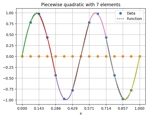
Here is the piecewise quadratic approximation of $f(x) = \sin(4 \pi x)$ .

Source

fun = lambda x: sin(4*pi*x)
xmin, xmax = 0.0, 1.0

N = 7         # no of elements
m = 2*N + 1   # no of data
x = linspace(xmin,xmax,m)
f = fun(x)

xe = linspace(xmin,xmax,500)
fe = fun(xe)

plot(x,f,'o',label='Data')
plot(x,0*f,'o')
plot(xe,fe,'k--',lw=1,label='Function')

# Local coordinates
xi = linspace(0,1,10)

phi0 = lambda x: 2*(x - 0.5)*(x - 1.0)
phi1 = lambda x: 4*x*(1.0 - x)
phi2 = lambda x: 2*x*(x - 0.5)

j = 0
for i in range(N):
    z  = x[j:j+3]
    h  = z[-1] - z[0]
    y  = f[j:j+3]
    fu = y[0]*phi0(xi) + y[1]*phi1(xi) + y[2]*phi2(xi)
    plot(xi*h + z[0], fu, lw=2)
    j += 2
title('Piecewise quadratic with '+str(N)+' elements')
legend(), xticks(x[::2]), grid(True), xlabel('x');

The vertical grid lines show the elements. The quadratic interpolant is shown in different color inside each element.

We can write the approximation in the form

p(x) = \sum_{k=0}^{2N} z_k \Phi_k(x), \qquad x \in [a,b]

(28)

where

z = (y_0, y_\half, y_1, \ldots, y_{N-1}, y_{N-1/2}, y_N) \in \re^{2N+1}

(29)

but this form should not be used in computations. For any $x \in [x_{i-1},x_i]$ only three terms in the sum survive reducing to the form (26).

6.9.3Piecewise degree $k$ interpolation¶

Consider a grid

a = x_0 < x_1 < \ldots < x_N = b

(30)

In each interval $[x_{i-1},x_i]$ we want to construct a degree $k$ polynomial approximation, so we need to know $k+1$ function values at $k+1$ distinct points

x_{i-1} = x_{i,0} < x_{i,1} < \ldots < x_{i,k} = x_i

(31)

Then the degree $k$ polynomial is given by

p(x) = \sum_{j=0}^k f(x_{i,j}) \phi_j\left( \frac{x-x_{i-1}}{h_i} \right)

(32)

where $\phi_j : [0,1] \to \re$ are Lagrange polynomials

\phi_j(\xi) = \prod_{l=0, l \ne j}^k \frac{\xi - \xi_l}{\xi_j - \xi_l}, \qquad \xi_l = \frac{x_{i,l} - x_{i-1}}{h_i}

(33)

with the property

\phi_j(\xi_l) = \delta_{jl}, \quad 0 \le j,l \le k

(34)

Since we choose the nodes in each interval such that $x_{i,0} = x_{i-1}$ and $x_{i,k} = x_i$ , the piecewise polynomial is continuous, but may not be differentiable.

6.9.4Error estimate in Sobolev spaces $^*$ ¶

The estimate we have derived required functions to be differentiable. Here we use weaker smoothness properties.

Proof 1

Since $\cts^\infty(0,1)$ is dense in $H^2(0,1)$ , it is enough to prove the error estimate for functions $f \in \cts^\infty(0,1)$ .

(1) If $x \in [x_j, x_{j+1}]$ then

\begin{aligned} f(x) - p(x) &= f(x) - \left[ f(x_j) + \frac{f(x_{j+1}) - f(x_j)}{x_{j+1} - x_j} (x - x_j) \right] \\ &= \int_{x_j}^x f'(t) \ud t - \frac{x - x_j}{x_{j+1} - x_j} \int_{x_j}^{x_{j+1}} f'(t) \ud t \\ &= (x-x_j) f'(x_j + \theta_x) - (x-x_j) f'(x_j + \theta_j), \quad {0 \le \theta_x \le x - x_j \atop 0 \le \theta_j \le h_j} \\ &= (x-x_j) \int_{x_j + \theta_j}^{x_j + \theta_x} f''(t) \ud t \end{aligned}

(37)

Squaring both sides and using $|x-x_j| \le h_j$

\begin{aligned} |f(x) - p(x)|^2 &\le h_j^2 \left[ \int_{x_j + \theta_j}^{x_j + \theta_x} f''(t) \ud t \right]^2 \\ &\le h_j^2 \left[ \int_{x_j}^{x_{j+1}} |f''(t)| \ud t \right]^2 \\ &\le h_j^3 \int_{x_j}^{x_{j+1}} |f''(t)|^2 \ud t \quad \textrm{by Cauchy-Schwarz inequality} \end{aligned}

(38)

Integrating on $[x_j,x_{j+1}]$

\int_{x_j}^{x_{j+1}} |f(x) - p(x)|^2 \ud x \le h_j^4 \int_{x_j}^{x_{j+1}} |f''(t)|^2 \ud t

(39)

Adding such an inequality from all the intervals

\begin{aligned} \norm{f-p}_{L^2(0,1)}^2 &\le \sum_j h_j^4 \int_{x_j}^{x_{j+1}} |f''(t)|^2 \ud t \\ &\le h^4 \sum_j \int_{x_j}^{x_{j+1}} |f''(t)|^2 \ud t \\ &= h^4 \norm{f''}_{L^2(0,1)}^2 \end{aligned}

(40)

we get the first error estimate.

(2) The error in derivative is

\begin{aligned} f'(x) - p'(x) &= f'(x) - \frac{f(x_{j+1}) - f(x_j)}{h_j} \\ &= \frac{1}{h_j} \int_{x_j}^{x_{j+1}}[f'(x) - f'(t)]\ud t \\ &= \frac{1}{h_j} \int_{x_j}^{x_{j+1}} \int_t^x f''(y) \ud y \ud t \end{aligned}

(41)

Squaring both sides

\begin{aligned} |f'(x) - p'(x)|^2 &= \frac{1}{h_j^2} \left( \int_{x_j}^{x_{j+1}} \int_t^x f''(y) \ud y \ud t \right)^2 \\ &\le \frac{1}{h_j^2} \left( \int_{x_j}^{x_{j+1}} \int_t^x |f''(y)| \ud y \ud t \right)^2 \\ &\le \frac{1}{h_j^2} \left( \int_{x_j}^{x_{j+1}} \int_{x_j}^{x_{j+1}} |f''(y)| \ud y \ud t \right)^2 \\ &= \left( \int_{x_j}^{x_{j+1}} |f''(y)| \ud y \right)^2 \\ &\le h_j \int_{x_j}^{x_{j+1}} |f''(y)|^2 \ud y \quad \textrm{by Cauchy-Schwarz inequality} \end{aligned}

(42)

Integrating with respect to $x$

\int_{x_j}^{x_{j+1}} |f'(x) - p'(x)|^2 \ud x \le h_j^2 \int_{x_j}^{x_{j+1}} |f''(y)|^2 \ud y

(43)

Adding such inequalities from each interval, we obtain the second error estimate.