Sympy

%config InlineBackend.figure_format = 'svg'
import numpy as np
import matplotlib.pyplot as plt

Let us import everything from sympy. We will also enable pretty printing.

from sympy import *
init_printing()

We must define symbols which will be treated symbolically

x = symbols('x')
type(x)

sympy.core.symbol.Symbol

Let us define an expression

f = x*sin(pi*x) + tan(pi*x)
print(f)

x*sin(pi*x) + tan(pi*x)

Differentiation. We can perform symbolic differentiation.

diff(f,x)

Compute second derivative

diff(f,x,2)

Product of two functions. Define a more complicated expression as product of two expressions

\[ h(x) = f(x) g(x) \]

and differentiate it

g = exp(x)
h = f*g
diff(h,x)

Function composition. Composition of two functions

\[ h(x) = (f \circ g)(x) = f(g(x)) \]

Apply this to the case \(f(x) = \sin(x)\), \(g(x) = \cos(x)\).

g = cos(x)
h = sin(g)
print('h =',h)
diff(h,x)

h = sin(cos(x))

If the two functions \(f,g\) have already been defined and we want to compose, then we can use substitution,

f = sin(x)
g = cos(x)
h = f.subs({'x':g})
print('h =',h)
diff(h,x)

h = sin(cos(x))

Integration. We can also compute indefinite integrals

print(f)
integrate(f,x)

sin(x)

We can get definite integrals.

integrate(f,(x,0,1))

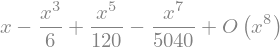
Taylor expansion. Compute Taylor expansion of \(f(x)\) around \(x=0\)

print(f)
series(f,x,0,8)

sin(x)

Compute Taylor expansion of \(h(x)\) around \(x=0\)

print(h)
series(h,x,0,8)

sin(cos(x))

Expression is not a function

p = (x + 1)/(x**2 + 2)

We cannot evaluate p at a numerical value. To do that, we can substitute the symbol x with a numerical value.

p.subs({'x':1})

p.subs({'x':1.0})

The result depends on whether we substitute with an integer or a float. You can substitute with a rational number like this

p.subs({'x':1//2})

For how to make python functions out of expressions, see below.

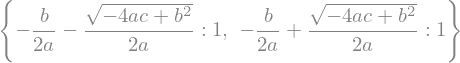
Compute roots

Let us find roots of quadratic equation

\[ a x^2 + b x + c = 0 \]

x, a, b, c = symbols('x a b c')
eq = a*x**2 + b*x + c
roots(eq,x)

x, a = symbols('x a')
eq = (x - a)**2
roots(eq,x)

Expand, factor, simplify

x, a = symbols('x a')
expand((x-a)**2)

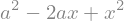
factor(x**2 - 2*a*x + a**2)

f = (x + x**2)/(x*sin(x)**2 + x*cos(x)**2)
simplify(f)

Get Latex code

x = symbols('x')
p = (cos(x)-sin(x))**3
expand(p)

print_latex(expand(p))

- \sin^{3}{\left(x \right)} + 3 \sin^{2}{\left(x \right)} \cos{\left(x \right)} - 3 \sin{\left(x \right)} \cos^{2}{\left(x \right)} + \cos^{3}{\left(x \right)}

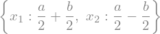
Solve a linear system

\[ x_1 + x_2 = a, \qquad x_1 - x_2 = b \]

x1, x2, a, b = symbols('x1 x2 a b')
e1 = x1 + x2 - a
e2 = x1 - x2 - b
solve([e1, e2],[x1,x2])

We can capture the result as a dictionary.

r = solve([e1, e2],[x1,x2])
print('x1 = ', r[x1])
print('x2 = ', r[x2])

x1 =  a/2 + b/2
x2 =  a/2 - b/2

Example: create Python function from sympy expression

Lets first define a function and get its derivative.

x = symbols('x')
f = x * sin(50*x) * exp(x)
g = diff(f,x)

We cannot evaluate f and g since they are not python functions. We first create Python functions out of the symbolic expressions and then plot them.

ffun = lambdify(x,f)
gfun = lambdify(x,g)

We can now evaluate these functions at some argument

print('f(1) =',ffun(1.0))
print('g(1) =',gfun(1.0))

f(1) = -0.7132087970679899
g(1) = 129.72606342238427

We can now use these to plot graphs of the functions

xx = np.linspace(0.0,1.0,200)
plt.figure(figsize=(9,4))
plt.subplot(121)
plt.plot(xx,ffun(xx))
plt.grid(True)
plt.title('f(x) = '+str(f))
plt.subplot(122)
plt.plot(xx,gfun(xx))
plt.grid(True)
plt.title('Derivative of f(x)');

Example: Truncation error of FD scheme

Approximate second derivative using finite difference scheme

\[ f''(x) \approx \frac{f(x-h) - 2 f(x) + f(x+h)}{h^2} \]

We perform Taylor expansion around \(x\) to find the error in this approximation: write

\[ f(x \pm h) = f(x) \pm h f'(x) + \frac{h^2}{2} f''(x) \pm \ldots \]

and simplify the rhs. This can be done by sympy.

x, h = symbols("x,h")
f = Function("f")
T = lambda h: (f(x-h) - 2*f(x) + f(x+h))/(h**2)
series(T(h), h, x0=0, n=6)

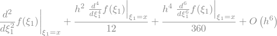
The above result shows that the FD formula is equal to

\[ \frac{f(x-h) - 2 f(x) + f(x+h)}{h^2} = f''(x) + \frac{h^2}{12} f^{(4)}(x) + \frac{h^4}{360} f^{(6)}(x) + O(h^6) \]

The leading error term is \(O(h^2)\)

\[ \textrm{error} = \frac{f(x-h) - 2 f(x) + f(x+h)}{h^2} - f''(x) = \frac{h^2}{12} f^{(4)}(x) + \frac{h^4}{360} f^{(6)}(x) + O(h^6) = O(h^2) \]

so that the formula is second order accurate.